16 Linear Regression
This chapter is under heavy development and may still undergo significant changes.
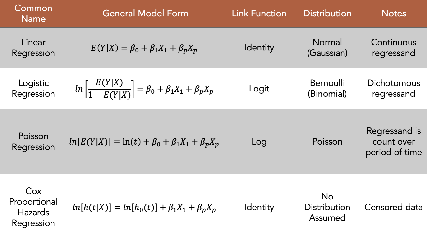
Figure 16.1: Four commonly used generalized linear models.
We introduced regression modeling generally in the introduction to regression analysis chapter. In this chapter, we will discuss fitting logistic regression models, a type of generalized linear model, to our data using R. In general, the logistic model is a good place to start when the regressand we want to model is dichotomous. We will begin by loading some useful R packages and simulating some data to fit our model to. We add comments to the code below to help you get a sense for how the values in the simulated data are generated. But please skip over the code if it feels distracting or confusing, as it is not the primary object of our interest right now.
# Load the packages we will need below
library(dplyr, warn.conflicts = FALSE)
library(broom) # Makes glm() results easier to read and work with
library(ggplot2)
library(meantables)
library(freqtables)
# Set the seed for the random number generator so that we can reproduce our results
set.seed(123)
# Set n to equal the number of people we want to simulate. We will use n
# repeatedly in the code below.
n <- 20
# Simulate a data frame with n rows
# The variables in the data frame are generic continuous, categorical, and
# count values. They aren't necessarily intended to represent any real-life
# health-related state or event
df <- tibble(
# Create a continuous regressor containing values selected at random from
# a normal distribution
x_cont = rnorm(n, 10, 1),
# Create a categorical regressor containing values selected at random from
# a binomial distribution with a 0.3 probability of success (i.e.,
# selecting a 1)
x_cat = rbinom(n, 1, .3),
# Create a continuous regressand that has a value that is equal to the value
# of x_cont plus or minus some random variation. The direction of the
# variation is dependent on the value of x_cat.
y_cont = if_else(
x_cat == 0,
x_cont + rnorm(n, 1, 0.1),
x_cont - rnorm(n, 1, 0.1)
),
# Create a categorical regressand that has a value selected at random from
# a binomial distribution. The probability of a successful draw from the
# binomial distribution is dependent on the value of x_cat.
y_cat = if_else(
x_cat == 0,
rbinom(n, 1, .1),
rbinom(n, 1, .5)
),
# Create a regressand that contains count data selected at random from
# a categorical distribution. The probability of a selecting each value from
# the distribution is dependent on the value of x_cat.
y_count = if_else(
x_cat == 0,
sample(1:5, n, TRUE, c(.1, .2, .3, .2, .2)),
sample(1:5, n, TRUE, c(.3, .3, .2, .1, .1))
)
)
# Print the value stored in df to the screen
df## # A tibble: 20 × 5
## x_cont x_cat y_cont y_cat y_count
## <dbl> <int> <dbl> <int> <int>
## 1 9.44 0 10.5 0 5
## 2 9.77 0 10.7 0 2
## 3 11.6 0 12.6 0 5
## 4 10.1 0 11.2 0 3
## 5 10.1 0 11.2 0 4
## 6 11.7 0 12.8 0 2
## 7 10.5 0 11.5 0 3
## 8 8.73 0 9.73 0 4
## 9 9.31 0 10.3 0 1
## 10 9.55 1 8.53 0 1
## 11 11.2 0 12.2 0 3
## 12 10.4 0 11.3 0 2
## 13 10.4 1 9.43 1 1
## 14 10.1 0 11.3 0 4
## 15 9.44 0 10.6 0 1
## 16 11.8 0 12.7 0 2
## 17 10.5 0 11.5 0 2
## 18 8.03 1 7.03 1 2
## 19 10.7 1 9.61 1 5
## 20 9.53 0 10.5 0 416.1 Categorical regressand continuous regressor
Now that we have some simulated data, we will fit and interpret a few different logistic models. We will start by fitting a logistic model with a single continuous regressor.
glm(
  y_cat  ~ x_cont,                   # Formula
  family = binomial(link = "logit"), # Family/distribution/Link function
  data   = df                        # Data
)
##
## Call: glm(formula = y_cat ~ x_cont, family = binomial(link = "logit"),
## data = df)
##
## Coefficients:
## (Intercept) x_cont
## 4.0428 -0.5798
##
## Degrees of Freedom: 19 Total (i.e. Null); 18 Residual
## Null Deviance: 16.91
## Residual Deviance: 16.17 AIC: 20.17This model isn’t the most interesting model to interpret because we are just modeling numbers without any context. However, because we are modeling numbers without any context, we can strip out any unnecessary complexity or biases from our interpretations. Therefore, in a sense, these will be the “purist”, or at least the most general, interpretations of the regression coefficients produced by this type of model. We hope that learning these general interpretations will help us to understand the models, and to more easily interpret more complex models in the future.
16.2 Categorical regressand categorical regressor
Next, we will fit a logistic model with a single categorical regressor. Notice that the formula syntax, the distribution, and the link function are the same for the single categorical regressor as they were for the single continuous regressor We just swap our x_cont for x_cat in the formula.
glm(
  y_cat  ~ x_cat,                    # Formula
  family = binomial(link = "logit"), # Family/distribution/Link function
  data   = df                        # Data
)
##
## Call: glm(formula = y_cat ~ x_cat, family = binomial(link = "logit"),
## data = df)
##
## Coefficients:
## (Intercept) x_cat
## -21.57 22.66
##
## Degrees of Freedom: 19 Total (i.e. Null); 18 Residual
## Null Deviance: 16.91
## Residual Deviance: 4.499 AIC: 8.49916.2.1 Interpretation
Intercept: The natural log of the odds of
y_catwhenx_catis equal to zero.x_catt: The average change in the natural log of the odds of
y_contwhenx_catchanges from zero to one.
Now that we have reviewed the general interpretations, let’s practice using logistic regression to explore the relationship between two variables that feel more like a scenario that we may plausibly be interested in.
16.3 Elder mistreatment example
set.seed(123)
n <- 100
em_dementia <- tibble(
  age = sample(65:100, n, TRUE),
  dementia = case_when(
    age < 70 ~ sample(0:1, n, TRUE, c(.99, .01)),
    age < 75 ~ sample(0:1, n, TRUE, c(.97, .03)),
    age < 80 ~ sample(0:1, n, TRUE, c(.91, .09)),
    age < 85 ~ sample(0:1, n, TRUE, c(.84, .16)),
    age < 90 ~ sample(0:1, n, TRUE, c(.78, .22)),
    TRUE ~ sample(0:1, n, TRUE, c(.67, .33))
  ),
  dementia_f = factor(dementia, 0:1, c("No", "Yes")),
  em = case_when(
    dementia_f == "No"  ~ sample(0:1, n, TRUE, c(.9, .1)),
    dementia_f == "Yes" ~ sample(0:1, n, TRUE, c(.5, .5))
  ),
  em_f = factor(em, 0:1, c("No", "Yes"))
)
em_dementia
## # A tibble: 100 × 5
## age dementia dementia_f em em_f
## <int> <int> <fct> <int> <fct>
## 1 95 0 No 0 No
## 2 79 0 No 0 No
## 3 78 0 No 0 No
## 4 67 0 No 1 Yes
## 5 78 0 No 0 No
## 6 89 0 No 0 No
## 7 90 0 No 0 No
## 8 91 0 No 0 No
## 9 69 0 No 0 No
## 10 91 1 Yes 1 Yes
## # ℹ 90 more rows16.3.1 Categorical regressor (dementia)
## # A tibble: 4 × 7
## row_var row_cat col_var col_cat n n_row percent_row
## <chr> <chr> <chr> <chr> <int> <int> <dbl>
## 1 dementia_f No em_f No 77 82 93.9
## 2 dementia_f No em_f Yes 5 82 6.10
## 3 dementia_f Yes em_f No 11 18 61.1
## 4 dementia_f Yes em_f Yes 7 18 38.9##
## Call: glm(formula = em_f ~ dementia_f, family = binomial(link = "logit"),
## data = em_dementia)
##
## Coefficients:
## (Intercept) dementia_fYes
## -2.734 2.282
##
## Degrees of Freedom: 99 Total (i.e. Null); 98 Residual
## Null Deviance: 73.38
## Residual Deviance: 61.72 AIC: 65.7216.3.2 Interpretation
Intercept: The natural log of the odds of
elder mistreatmentamong people who do not have dementia is -2.734. (Generally not of great interest or directly interpreted)dementia_fYes: The average change in the natural log of the odds of
elder mistreatmentamong people with dementia compared to people without dementia.
## # A tibble: 1 × 2
## intercpet dementia_or
## <dbl> <dbl>
## 1 0.0650 9.80- dementia_fYes: People with dementia have 9.8 times the odds of
elder mistreatmentamong compared to people without dementia.
em_dementia_ct <- matrix(
c(a = 7, b = 11, c = 5, d = 77),
ncol = 2,
byrow = TRUE
)
em_dementia_ct <- addmargins(em_dementia_ct)
dimnames(em_dementia_ct) <- list(
Dementia = c("Yes", "No", "col_sum"), # Row names
EM = c("Yes", "No", "row_sum") # Then column names
)
em_dementia_ct## EM
## Dementia Yes No row_sum
## Yes 7 11 18
## No 5 77 82
## col_sum 12 88 100incidence_prop <- em_dementia_ct[, "Yes"] / em_dementia_ct[, "row_sum"]
em_dementia_ct <- cbind(em_dementia_ct, incidence_prop)
em_dementia_ct## Yes No row_sum incidence_prop
## Yes 7 11 18 0.38888889
## No 5 77 82 0.06097561
## col_sum 12 88 100 0.12000000incidence_odds <- em_dementia_ct[, "incidence_prop"] / (1 - em_dementia_ct[, "incidence_prop"])
em_dementia_ct <- cbind(em_dementia_ct, incidence_odds)
em_dementia_ct## Yes No row_sum incidence_prop incidence_odds
## Yes 7 11 18 0.38888889 0.63636364
## No 5 77 82 0.06097561 0.06493506
## col_sum 12 88 100 0.12000000 0.13636364## [1] 9.8# Alternative coding
em_dementia %>%
  freq_table(dementia_f, em_f) %>%
select(row_var:n_row, percent_row) %>%
filter(col_cat == "Yes") %>%
mutate(
prop_row = percent_row / 100,
odds = prop_row / (1 - prop_row)
) %>%
summarise(or = odds[row_cat == "Yes"] / odds[row_cat == "No"])## # A tibble: 1 × 1
## or
## <dbl>
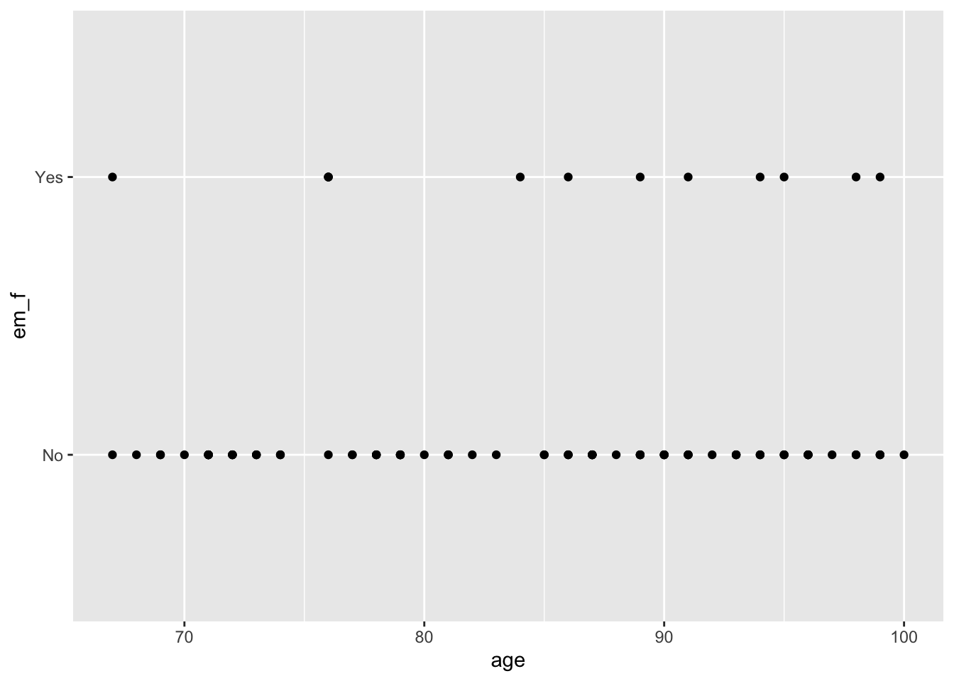
## 1 9.816.3.3 Continuous regressor (age)
## # A tibble: 2 × 11
##   response_var group_var group_cat     n  mean    sd   sem   lcl   ucl   min   max
##   <chr>        <chr>     <fct>     <int> <dbl> <dbl> <dbl> <dbl> <dbl> <int> <int>
## 1 age          em_f      No           88  84    9.57  1.02  82.0  86.0    67   100
## 2 age em_f Yes 12 85.9 10.3 2.96 79.4 92.4 67 99##
## Call: glm(formula = em_f ~ age, family = binomial(link = "logit"),
## data = em_dementia)
##
## Coefficients:
## (Intercept) age
## -3.80001 0.02127
##
## Degrees of Freedom: 99 Total (i.e. Null); 98 Residual
## Null Deviance: 73.38
## Residual Deviance: 72.96 AIC: 76.9616.3.4 Interpretation
Intercept: The natural log of the odds of
elder mistreatmentamong people who do not have dementia is -3.80. (Generally not of great interest or directly interpreted)age: The average change in the natural log of the odds of
elder mistreatmentfor each one-year increase in age is 0.02.
glm(
  em_f  ~ age,
  family = binomial(link = "logit"),
  data   = em_dementia
) %>%
broom::tidy(exp = TRUE, ci = TRUE)## # A tibble: 2 × 5
## term estimate std.error statistic p.value
## <chr> <dbl> <dbl> <dbl> <dbl>
## 1 (Intercept) 0.0224 2.83 -1.34 0.179
## 2 age 1.02 0.0328 0.648 0.517## [1] -1.6911## [1] -1.66983## [1] 0.02127## [1] 1.021498## # A tibble: 7 × 5
## age dementia dementia_f em em_f
## <int> <int> <fct> <int> <fct>
## 1 71 0 No 0 No
## 2 71 0 No 0 No
## 3 71 0 No 0 No
## 4 70 0 No 0 No
## 5 71 0 No 0 No
## 6 71 0 No 0 No
## 7 71 0 No 0 No