12 Effect-measure Modification
This chapter is under heavy development and may still undergo significant changes.
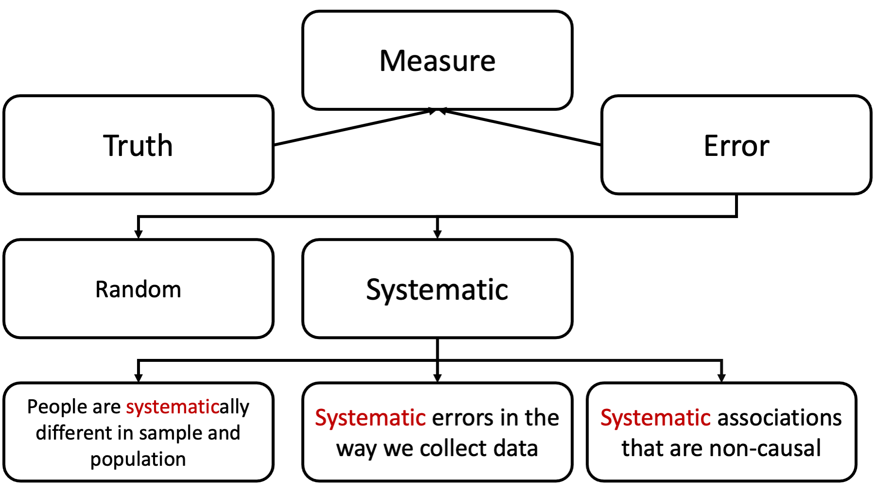
Unlike the past few weeks, effect modification is NOT error in our measure of the truth. It’s not something we are trying to eliminate; rather, it’s something we are trying to understand.
In some ways, this is a very simple lesson. In other ways, it can be very confusing (although, I’m going to try to help with that). For starters, the term “effect modification” is used inconsistently by different people and different resources, and other terms are often used to mean the same thing effect modification means (sometimes incorrectly). Additionally, the term “effect modification” is sometimes used to describe concepts that are technically distinct from effect modification.
Some of the other terms you may hear are effect-measure modification, heterogeneity of effects, subgroup effects, and interaction.
We will discuss the ways in which you can draw distinctions between these terms soon, but first I want to make sure we develop an intuition for what effect modification is.
Before doing so, however, I should probably specifically point out two things that effect modification is NOT.
First, unlike confounding, effect modification does not necessarily require a causal context to have meaning. Effect modification of non-causal relationships are all over the place and may even be useful in predictive modeling. Therefore, it’s probably worth specifically saying that the term ”effect” in “effect modification” seems to imply that we are only dealing with causal relationships, but that isn’t the case. Here, we are not necessarily using the word “effect” in the technical sense of cause and effect.
Second, effect modification is not currently considered to be the same thing, conceptually, as confounding. Let me be clear, every source I read while preparing this module describes effect modification and confounding as different things.
Having said that, recent methodological work is beginning to blur the lines between the two. I won’t talk much about this because I don’t want to confuse you, but you can read the citation at the bottom of this slide for more details if you’re interested. For now, you should definitely say that confounding and effect modification are different things on your exams and whatnot.
With those caveats out of the way, let’s start with a simple idea. There is some relationship between two variables, X and Y. Here, we are showing a causal relationship, but as I said earlier, effect modification can be present in non-causal relationships as well.
To make this more concrete, we’ll also assign labels to the variables X and Y.

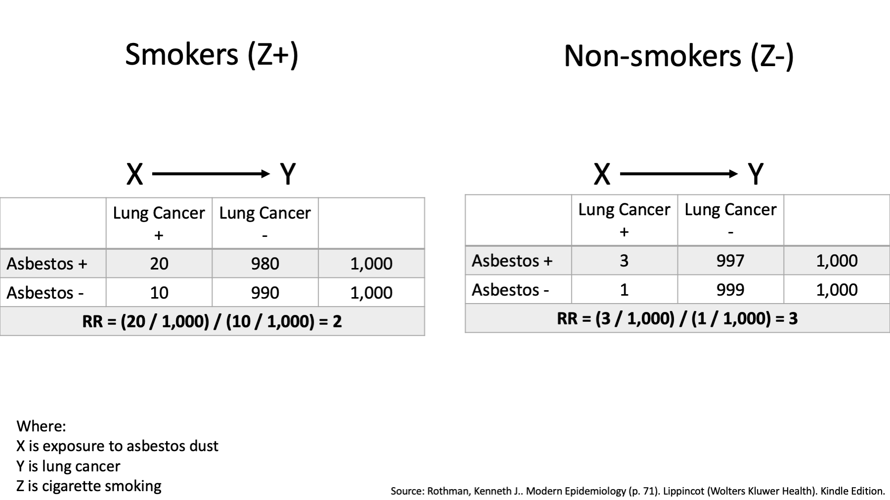
Specifically, I’m going to borrow a hypothetical example from the book Modern Epidemiology. In this example, the variable X represents exposure to asbestos dust and Y represents lung cancer.
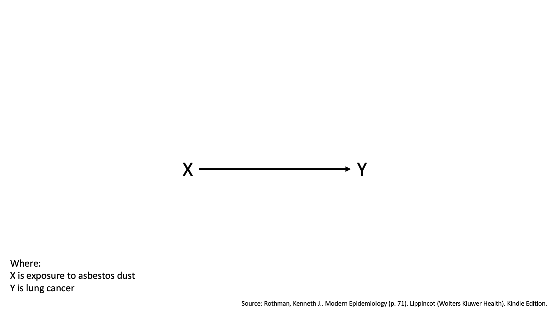
The causal DAG above tells us that exposure to asbestos dust causes lung cancer. It also tells us that we should expect a statistical association between exposure to asbestos dust and lung cancer in our data.
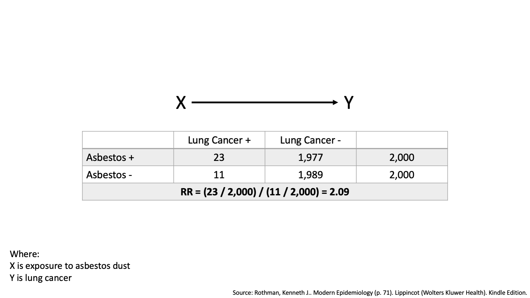
Now, suppose we examine the average 10-year risk of lung cancer in an occupational setting and find that the risk among the workers who were exposed to asbestos dust was 2.09 times the risk among workers who were not exposed to asbestos dust over the 10-year period. That’s an interesting finding, and completely consistent with our DAG.
But, suppose we believe that smoking cigarettes might have played an important role in the development of lung cancer as well. In this case, we don’t necessarily believe that we are giving credit to Asbestos that belongs to smoking (remember last week, not a common cause, no open backdoor path); rather, we think that asbestos exposure is more likely to produce lung cancer in smokers than it is in non-smokers. How might we evaluate that hypothesis?
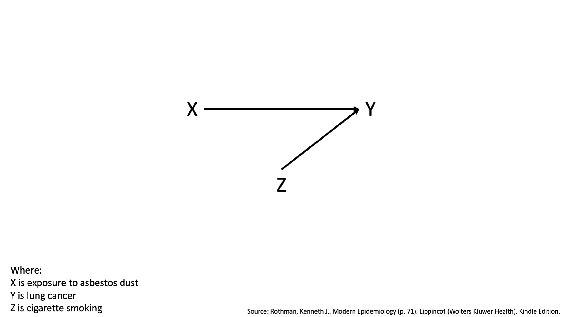
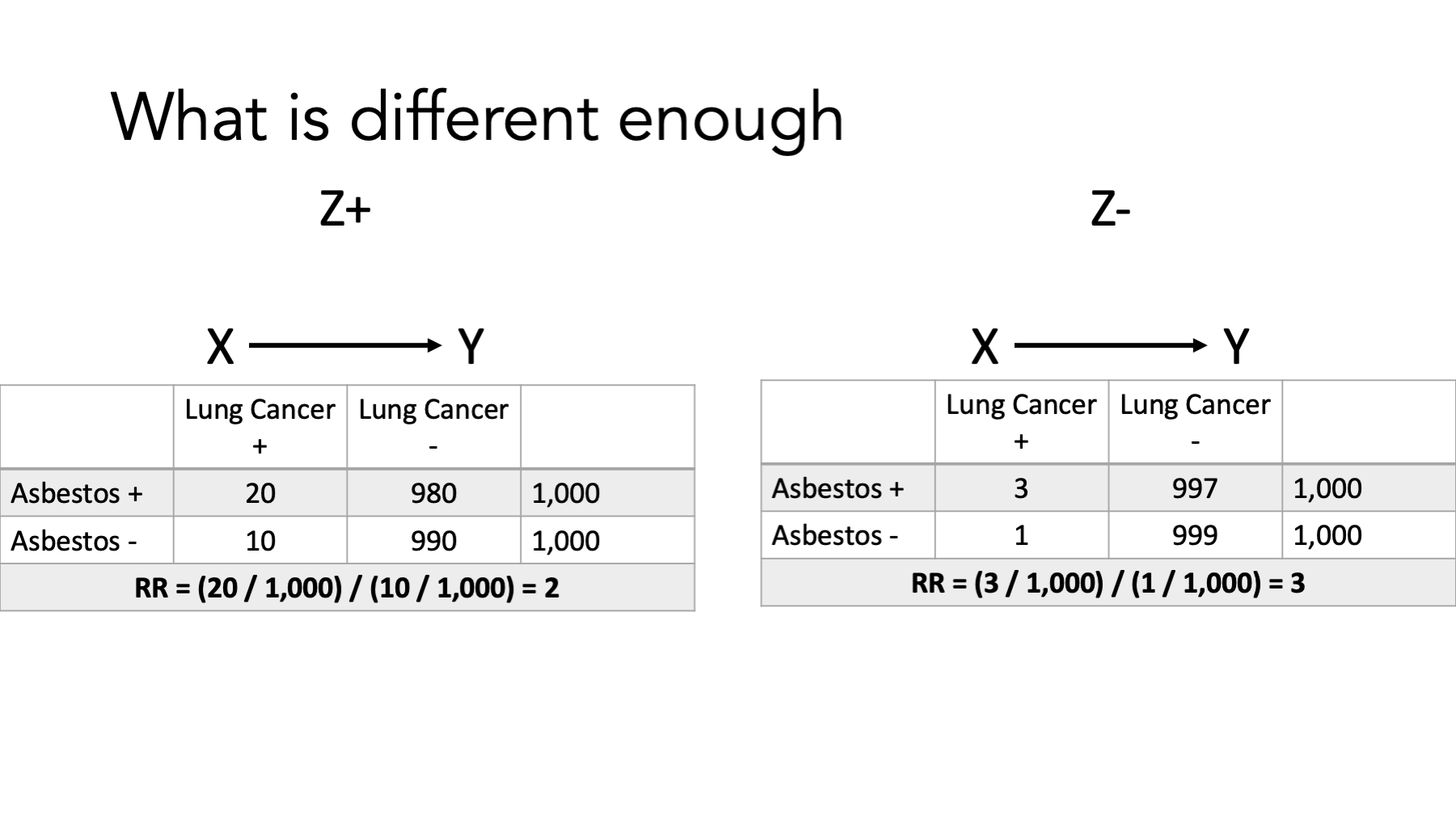
Well, one way to do that would be estimate the effect of asbestos dust on lung cancer only among people who smoked (represented here by Z+), estimate the effect of asbestos dust on lung cancer only among people who didn’t smoked (represented here by Z-), and then see if our estimates of the effect are the same or different.
That’s exactly what we’ve done here. Let’s pause and take a look.
What are the measures we are using to characterize the effect of asbestos dust on lung cancer? Risk ratios (relative risks).
Are the estimates of the effect (i.e., the risk ratios) the same or different?
They are different, right? Among smokers the risk ratio is 2. That is, among smokers, those who were exposed to asbestos dust had 2 times the risk of lung cancer compared to smokers who were not exposed to asbestos dust. Among non-smokers the risk ratio is 3. That is, among non-smokers, those who were exposed to asbestos dust had 3 times the risk of lung cancer compared to non-smokers who were not exposed to asbestos dust. And that’s it. That’s the big idea. The measure of the effect of asbestos on lung cancer is not the same in smokers and non-smokers. From that point of view, I think it’s a pretty simple idea.
I’d also like you to notice that we did not discuss the relationship between smoking and lung cancer at all on this slide. We discussed the relationship between asbestos and lung cancer within groups that where based on smoking status.
Finally, some of you may have noticed that the risk ratio is smaller in the non-smoking group than the smoking group and be curious as to why. We’ll come back to that.

At this point, I hope you have developed an intuition about what effect modification is. Before getting into greater detail about effect modification is, I’m going to take a detour through how it is distinct from interaction. I’m warning you now, the distinction can seem subtle and a little difficult to wrap your mind around, but I will do my best to make it practically digestible.
12.1 Difference between effect modification and effect measure modification?
This first definition of effect modification comes from A Dictionary of Epidemiology. Notice that this definition closely matches our example about asbestos and lung cancer. It also directly tells us that effect-measure modification is a synonym.
EFFECT MODIFICATION (Syn: effect-measure modification) Variation in the selected effect measure for the factor under study across levels of another factor. See also INTERACTION (Porta, Miquel. A Dictionary of Epidemiology (p. 76). Oxford University Press. Kindle Edition).
“Epidemiologists often use the term effect modification to mean what is described here as effect-measure modification. The addition of the word measure to the phrase is intended to emphasize the dependence of this phenomenon on the choice of the effect measure and its consequent ambiguity. One cannot speak in general terms about the presence or absence of effect modification, any more than one can speak in general terms about the presence or absence of clouds in the sky, without being more specific as to the details. For clouds in the sky, the details would include the geographic area, the time, and perhaps what is meant by a cloud. In the case of effect-measure modification, the details are in the choice of effect measure.” (Rothman, Kenneth J.. Epidemiology: An Introduction (p. 200). Oxford University Press. Kindle Edition).
In my opinion, the overall message is that effect-measure modification is a more precise way of saying effect modification.
“Since one cannot generally state that there is, or there is not, effect modification without referring to the effect measure being used (e.g., risk difference, risk ratio), some authors use the term effect-measure modification, rather than effect modification, to emphasize the dependence of the concept on the choice of effect measure.” (Hernán MA, Robins JM. Causal Inference: What If. CRC Press; 2020).
How about our friend Miguel Hernan? What does he have to say about the two?
My reaction to this quote is very similar to my reaction after reading Rothman’s quote The overall message is that effect-measure modification is a more precise way of saying effect modification.
”Effect-measure modification (heterogeneity): Suppose we divide our population into two or more categories or strata. In each stratum, we can calculate an effect measure of our choosing. These stratum-specific effect measures may or may not equal one another.” (Rothman, Kenneth J.. Modern Epidemiology (p. 61). Lippincot (Wolters Kluwer Health). Kindle Edition).
“The term effect modification is also ambiguous, and we again advise more precise terms such as risk-difference modification or risk-ratio modification, as appropriate.” (Rothman, Kenneth J.. Modern Epidemiology (p. 74). Lippincot (Wolters Kluwer Health). Kindle Edition).
Finally, let’s see what the very popular textbook, Modern Epidemiology, has to say about it.
Again, it seems like we should be able to use effect modification and effect-measure modification fairly interchangeably. They do go on to say, however, that the term effect modification is too ambiguous and advise using very specific terms that indicate the exact measure that is being modified. We’ll see why they say this shortly.
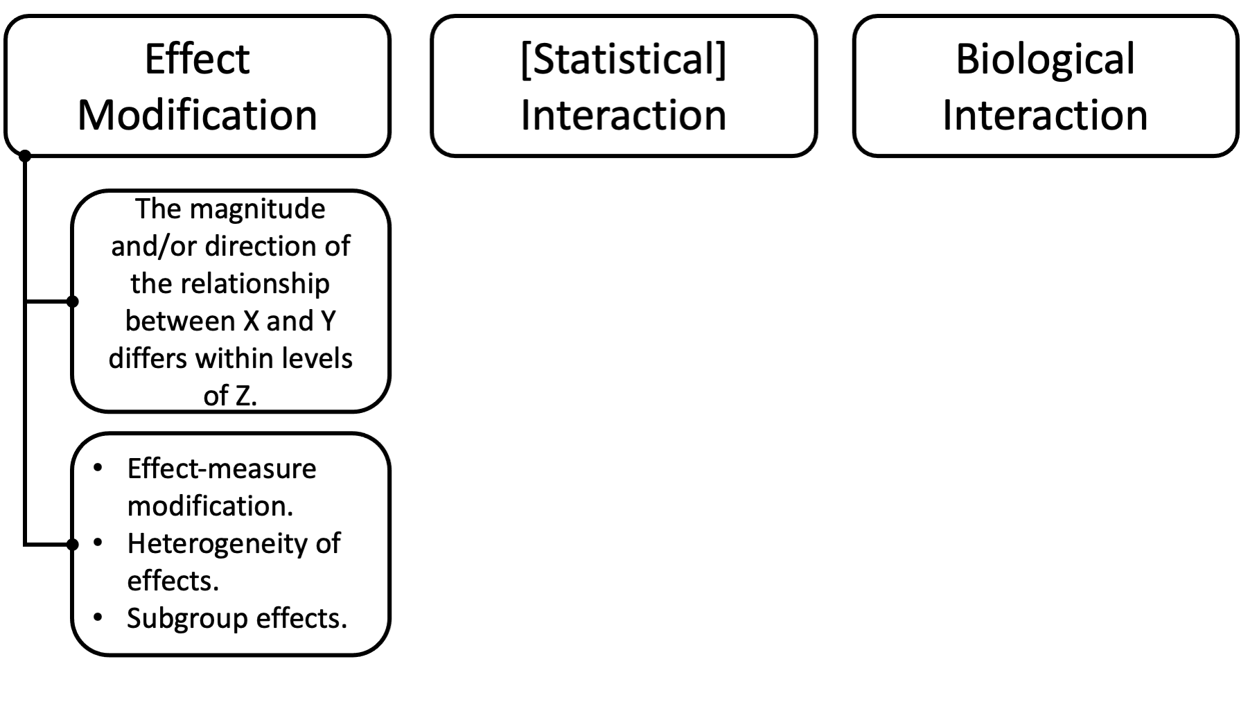
So, it seems to me that effect-measure modification can reasonably be thought of as a synonym for effect modification, along with the terms heterogeneity of effects and subgroup effects.
All of these things describe a situation in which the magnitude and/or direction of the relationship between two variables, X and Y, is different within levels of a third variable, Z. This is the same situation we saw in the asbestos and lung cancer example.
However, that still leaves us needing to distinguish between effect modification and statistical and biological interaction.
12.2 Difference between effect modification and statistical interaction
The formal distinction between effect modification and statistical interaction is sort subtle, pretty technical, and probably beyond the scope of this course. A variable Q is said to be an effect modifier on the causal risk difference scale for the effect of E on D, conditional on X, if Q is not an effect of E and if there are 2 levels of E, e0 and e1, and 2 levels of Q, q0 and q1, and some x, such that E[De1 | Q = q1, X = x] - E[De0 | Q = q1, X = x] ≠ E[De1 | Q = q0, X = x] - E[De0 | Q = q0, X = x] E[De1 | Q = q1] - E[De0 | Q = q1] ≠ E[De1 | Q = q0] - E[De0 | Q = q0]
There is said to be an interaction on the causal risk difference scale between the effects of E and Q on D, conditional on X, if there are 2 levels of E, e0, and e1, and 2 levels of Q, q0, and q1, such that for some x, E[De1q1 | X = x] - E[De0q1 | X = x] ≠ E[De1q0 | X = x] - E[De0q0 | X = x] E[De1q1] - E[De0q1] ≠ E[De1q0] - E[De0q0]
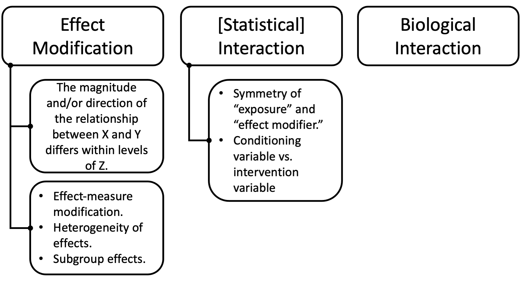
Note there is an asymmetry (i.e., one is more “important” than the other) between E and Q in the definition of effect modification: only the effect of one of the 2 exposures is principally in view, namely the effect of E on D. The role of the other exposure Q in the definition simply concerns whether the effect of primary interest varies across strata of this other exposure Q. In contrast to this definition of effect modification, the roles of E and Q in the definition of interaction are symmetric.
Note further that in Definition 2, interventions on both E and Q are being considered. In the definition given for effect modification, only interventions on exposure E were being considered (setting E to e1 in contrast to setting E to e0) whereas interventions were not being considered for Q; the role of Q in Definition 1 for effect modification was that of a conditioning variable. Thus, Q is a conditioning variable in the definition of effect modification, and an intervention variable in the definition of interaction.
It has been shown that interactions (even causal interactions as given in Definition 2) on the risk difference or risk ratio or odds ratio scale need not correspond to interactions in any biologic or mechanistic sense.
So this might be one of those times when you do the same thing either way, but your interpretation may be different.
Here’s another way to think about it that may be useful.
If we randomize one intervention and then see if its effects are different based on some participant characteristic, then that’s effect modification.
If we randomize people to get two different treatments and we assess whether those two interventions have synergistic effects that’s causal interaction.
Problem is that a statistical interaction in a regression model can’t distinguish between these two distinct causal concepts.
There are more advanced analytic methods like standardization by weights that can distinguish them, but that’s beyond the scope of an MPH.
As we saw, previously (and may or may not fully understand) statistical interaction is distinct from effect modification in its mathematical definition. I think the takeaway messages that are important for us are given here.
But, if you find this super confusing, then just let it go for now. You aren’t going to be tested on it. And, in practice, the terms effect modification and interaction are often used synonymously.
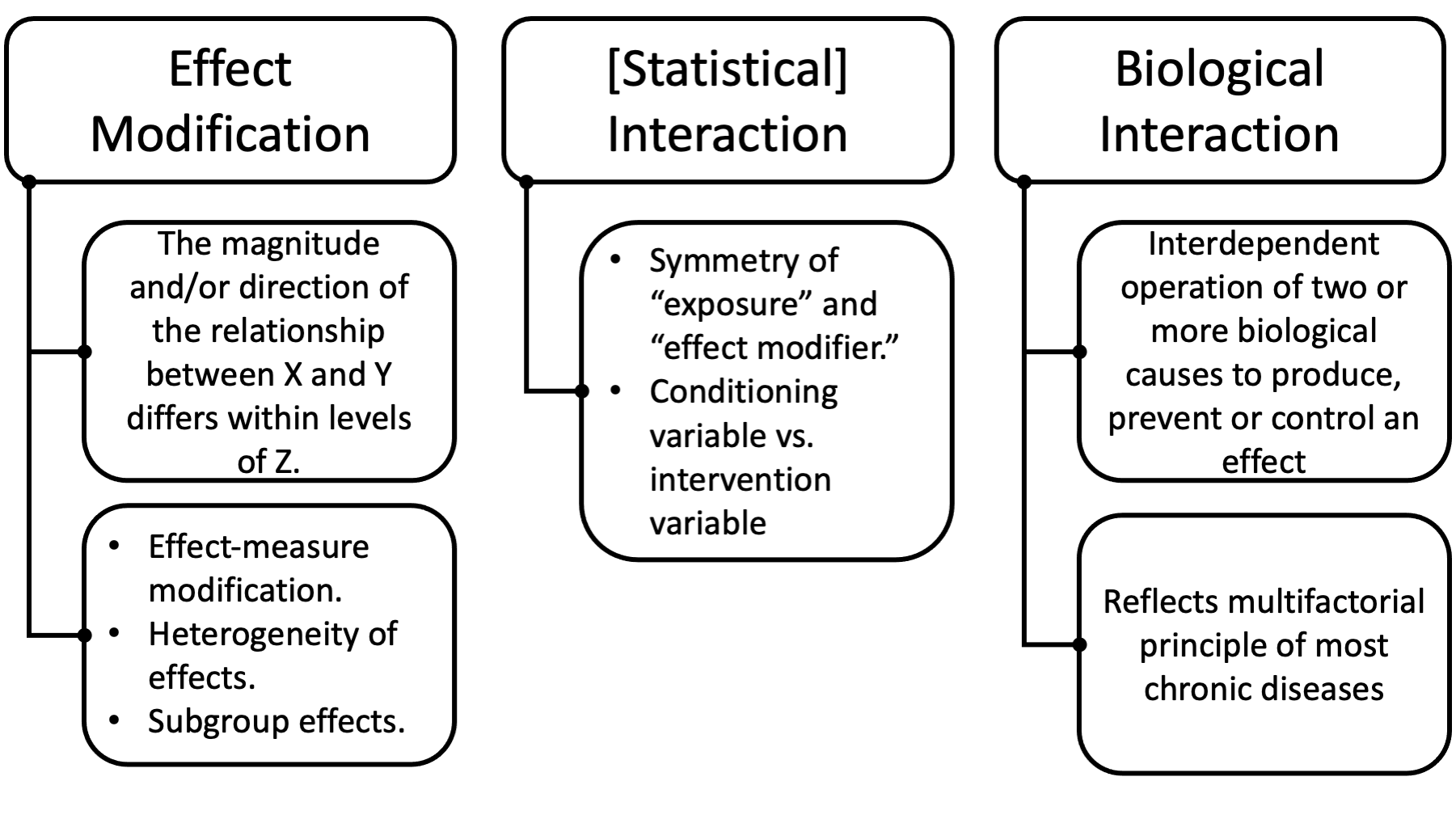
03Finally, there is yet another distinct form of interaction called biological interaction.
For biological interaction, you can think of the sufficient-component cause model. If a sufficient causal pie has more than one component cause, then both component causes interact to produce the outcome.
12.3 Assessing (exploring) effect modification
Now that we have (hopefully) detangled and clarified some terminology, let’s dive slightly deeper into some analytic details.
“A major point about effect-measure modification is that, if effects are present, it will usually be the case that no more than one of the effect measures discussed above will be uniform across strata. In fact, if the exposure has any effect on an occurrence measure, at most one of the ratio or difference measures of effect can be uniform across strata.” (Rothman, Kenneth J.. Modern Epidemiology (p. 61). Lippincot (Wolters Kluwer Health). Kindle Edition.)
Let me just start by saying something that may seem somewhat controversial or confusing. In one sense effect modification will almost always be present. So, when we talk about assessing effect modification, we typically aren’t talking about assessing if it is there or not. We are talking about investigating its scale and magnitude, and then thinking through the implication of what we find out about its scale and magnitude. For that reason, I kind of prefer to the term exploring to assessing.
The quote above tells us that effect modification, to some extent, will nearly always be present. This quote tells us something about why that’s the case. It is the case because when effect modification is not present on one scale, in many circumstances it must be present on another scale.
If you are interested, you can see the mathematical proof in the Modern Epidemiology textbook. We are just going to take this statement a face value for the purposes of this course. A more important question for us is, “what do we mean by scale?”
“Thus, when both factors have effects, absence of statistical interaction on any particular scale necessarily implies presence of statistical interaction on many other scales” (Rothman, Kenneth J.. Modern Epidemiology (p. 61). Lippincot (Wolters Kluwer Health).
Remember back to the module on measures of outcome occurrence? We talked about measuring outcome occurrence on one of two scales – additive or multiplicative.
We talked about risk differences being an additive measure of effect that is especially useful in the context of understanding disease burden and public health planning.
Additive - Examination of risk difference - Joint effects compared to the sum of individual effects - Linear regression: 𝑦= 𝛽0+ 𝛽1x1+β2𝑥2
Additionally, we’ve talked a lot about ratio measures of effect including risk ratios, rate ratios, and odds ratios. These are typically described as being most useful for understand disease etiology
Multiplicative - Examination of ratio measures of effect - Joint effects compared to the product of individual effects - Logistic regression: odds = 𝑝/(1−𝑝)= ℯ^𝛽0 ∗ℯ^𝛽1𝑥1 * ℯ^𝛽2𝑥2
As a side note, there are other regression measures of effect that we haven’t yet learned about. These measures of effect may also be classified as additive or multiplicative. We aren’t going to discuss them today. For now, just know that they exist, and they can also be classified in this way.
When we use the measure types you see here to quantify outcome occurrence, we say that we are measuring occurrence on either an additive or multiplicative scale.
When we compare the measure types you see here to explore effect modification, we say that we are exploring (or assessing) effect modification on either a additive or multiplicative scale.
When we make those comparisons, we can find multiple different types of relationships.
Qualitative effect modification - The exposure effect can be seen in one strata, but not in another - RRmen = 1.0, RRwomen = 2.0 - RDmen = 0.0 / 1,000, RDwomen = 2.0 / 1,000
- The exposure is helpful in one strata, but harmful in another
- RRmen = 0.5, RRwomen = 2.5
- RDmen = -1.0 / 1,000, RDwomen = 2.0 / 1,000
Quantitative effect modification - The exposure is harmful (or helpful) in both strata, but the magnitude is different - RRmen = 2.0, RRwomen = 6.0 - RDmen = 2.0 / 1,000, RDwomen = 10.0 / 1,000
In the presence of qualitative effect modification, additive effect modification implies multiplicative effect modification, and vice versa. In the absence of qualitative effect modification, however, one can find effect modification on one scale (e.g., multiplicative) but not on the other (e.g., additive).
-Hernan
And, in this module we learn about two different methods for exploring effect modification, which can typically be used to explore effect modification on either scale.
We can explore homogeneity of effects across one or more other variables. Although, there are some exceptions. For example, in a case-control study, the homogeneity strategy can generally be used to assess effect modification on the multiplicative scale only (Szklo, Moyses,Nieto, F. Javier. Epidemiology (Kindle Locations 5776-5777). Jones & Bartlett Learning. Kindle Edition).
We can also explore differences between observed and expect joint effects.
Homogeneity of Effects - Are the effects of our exposure the same with strata of the effect modifier?
Observed and Expected Joint Effects - The observed joint effects of the risk factor and third factor differ from that expected on the basis of their independent effects.
12.3.1 Homogeneity of Effects
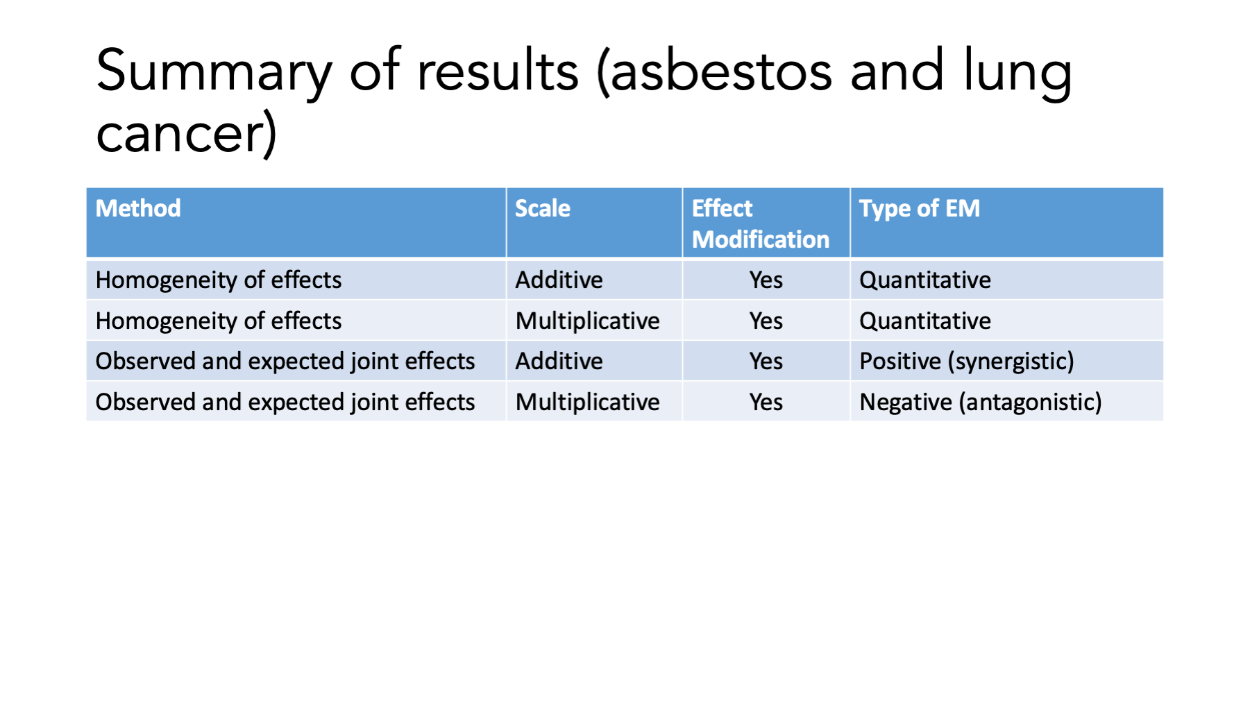
This is the example from the beginning of this discussion. Did we explore effect modification here on an additive or multiplicative scale? Multiplicative (RR).
Which method did we use to to explore effect modification – homogeneity of effects or comparing observed and expected joint effects? Homogeneity of effects.
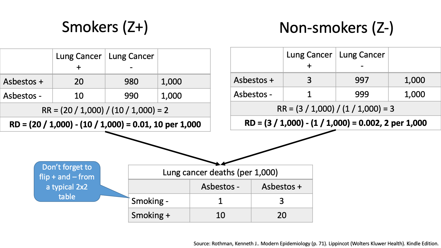
However, we could have also explored effect modification on the additive scale by comparing risk differences between smokers and non-smokers like this.
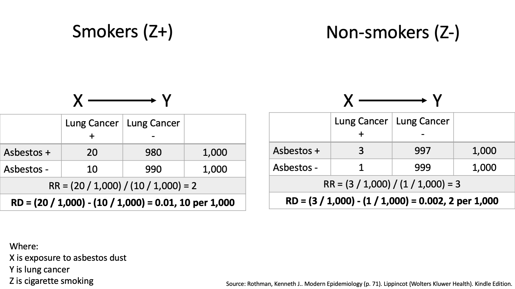
We can see that the risk is 20 / 1,000 among asbestos workers who smoked, and it is 10 / 1,000 in workers who smoked and did not work with asbestos.
We can also see that among nonsmoking asbestos workers, this risk is 3 / 1,000, and the corresponding risk is 1 / 1,000 in nonsmoking workers who did not work with asbestos.
The risk ratio association between asbestos exposure and lung cancer is then 2 in smokers, less than the risk ratio of 3 in non-smokers.
Further, the risk difference is 0.01 or 10 per 1,000 in smokers, greater than the risk difference of 0.002 or 2 per 1,000 among non-smokers.
Thus, when using the ratio measure, it appears that the association between asbestos exposure and lung cancer risk is greater in nonsmokers than smokers. When using the difference measure, however, it appears that the association is considerably less for nonsmokers than for smokers.
Rothman, Kenneth J.. Modern Epidemiology (p. 71). Lippincot (Wolters Kluwer Health). Kindle Edition.
Highlight:
Overall, cancer is higher in smokers (20 and 10 vs. 3 and 1) The RR is different within strata – effect modification on the multiplicative scale. The RD is different within strata – effect modification on the additive scale. The RR is higher in Non-smokers (When it isn’t smoking, it has to be something). The RD is higher in smokers (Smoking is bad. Smoking and asbestos is really bad).
Main idea: Not the same within strata.

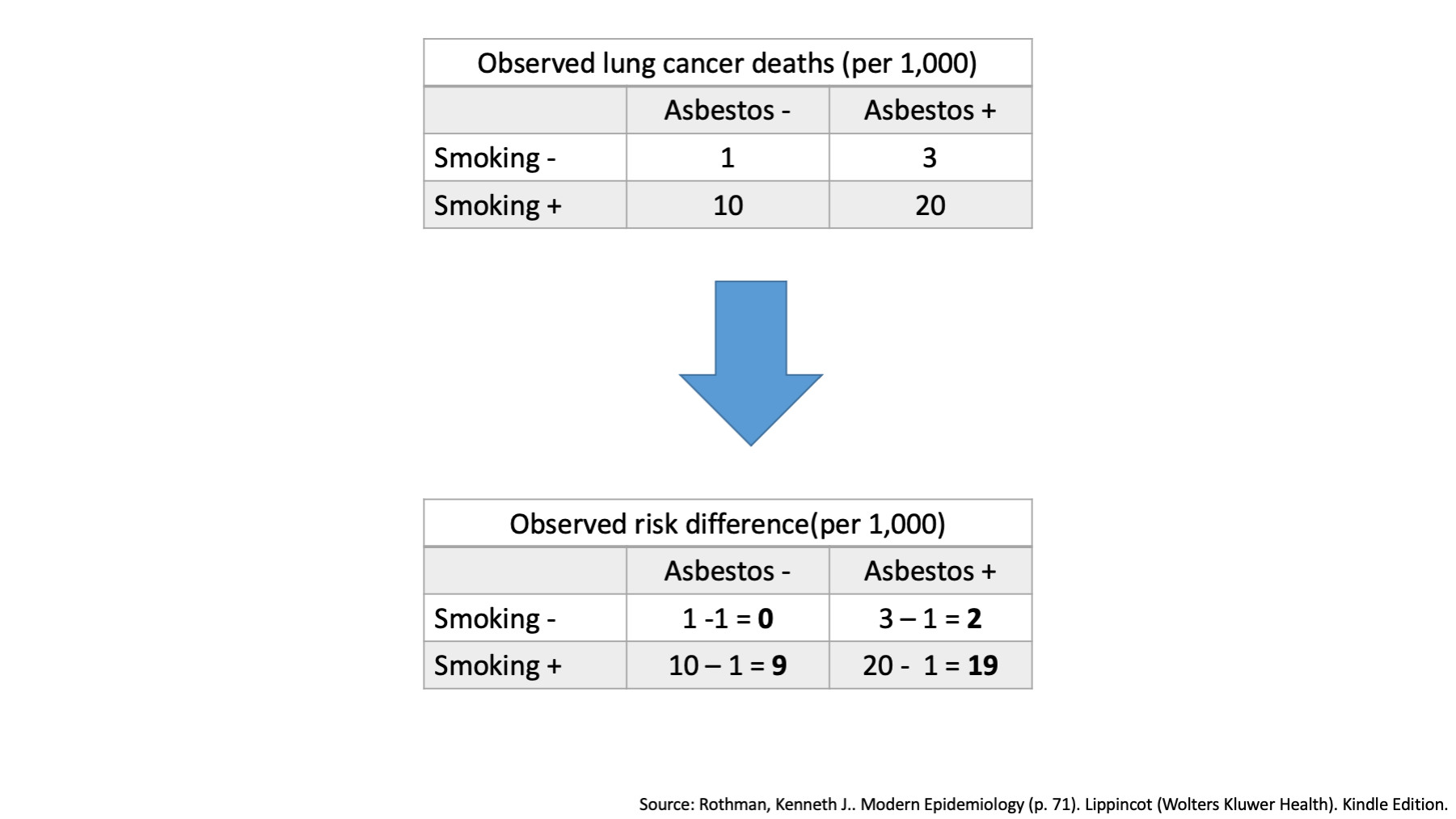
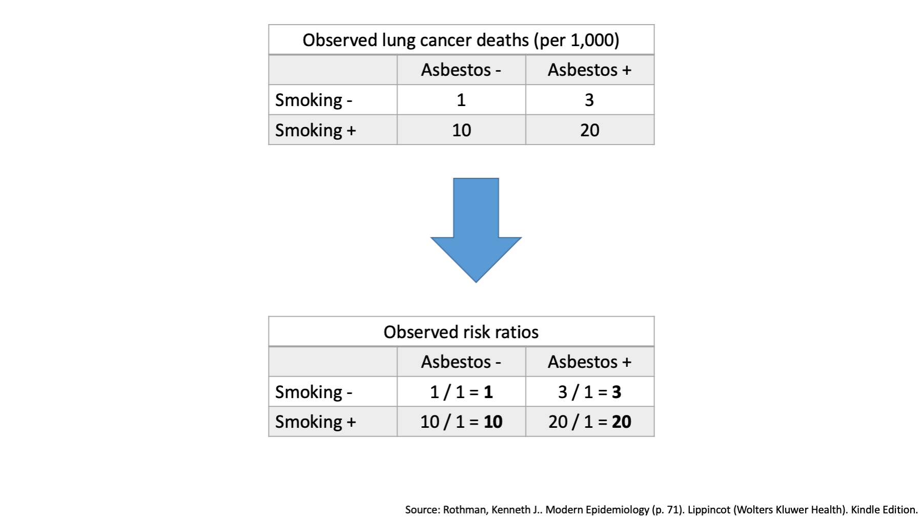
We can also compare joint and expected effects. First, let’s use our data to create a new table that includes lung cancer deaths by exposure status – both exposure to smoking and exposure to asbestos dust.
How many lung cancer deaths occurred among workers who did not smoke and were not exposed to asbestos? 1
How many lung cancer deaths occurred among workers who did not smoke, but were exposed to asbestos? 3
How many lung cancer deaths occurred among workers who smoked and were not exposed to asbestos? 10
Finally, how many lung cancer deaths occurred among workers who smoked and were exposed to asbestos? 20
Now, when there is no effect modification, we expect the combined effects of our two exposures to simply equal the combination of their individual effects. On an additive scale, we combine the individual effects by addition.
In the top left corner of our table, we see that one person died who did not have exposure to smoking or asbestos. This tells us that there must be at least one sufficient cause set for lung cancer that includes neither smoking nor asbestos. We sometimes call that our baseline risk with respect to smoking and asbestos. Another way to think about it is an estimate of what lung cancer risk would be if we magically got rid of smoking and asbestos, but everything else stayed the same. We will designate this cell the reference cell.
The top right corner of our table tells us about the risk of lung cancer among people exposed to asbestos in the absence of smoking.
The bottom left corner of our table tells us about the risk of lung cancer among smokers in the absence of asbestos exposure.
Finally, the bottom right corner of our table tells us about the risk of lung cancer among people who smoked and were exposed to asbestos.
Remember, that we said that when there is no effect modification, we expect the combined effects of our two exposures to simply equal the combination of their individual effects. On an additive scale, the effect of interest could be the risk difference.
The observed risk difference in the second table represents the differences in the observed absolute incidence between each category and the reference category.
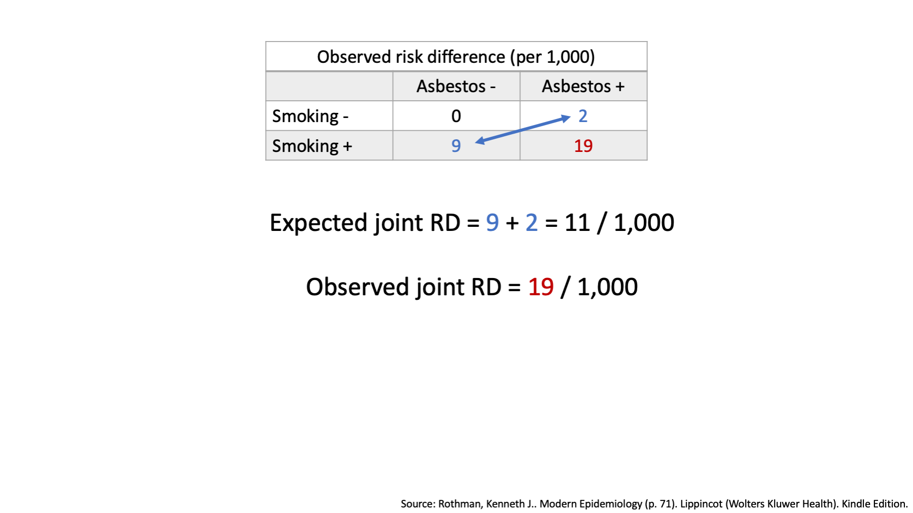
Once again, when there is no effect modification, we expect the combined effects of our two exposures to simply equal the combination of their individual effects. On an additive scale, we combine the individual effects by addition.
We already decided that the individual effects of smoking and of asbestos on an additive scale were located in the corners of our table.
We also said that when we are exploring effect modification on an additive scale, we combine the individual effects by addition.
Therefore, the expected joint risk difference of 11 / 1,000, which is lower than the observed joint risk difference of 19 / 1,000. This is effect modification on the additive scale.
Now, let’s explore multiplicative interaction using the comparison of observed and expected joint effects method.
12.3.2 Observed and Expected Joint Effects
The first step, using our data to create a new table that includes lung cancer deaths by exposure status – both exposure to smoking and exposure to asbestos dust is the same as before.
Once again, when there is no effect modification, we expect the combined effects of our two exposures to simply equal the combination of their individual effects. On an multiplicative scale, we combine the individual effects by multiplication.
In the top left corner of our table, we see that one person died who did not have exposure to smoking or asbestos. This cell will still be designated the reference cell.
Remember, that we said that when there is no effect modification, we expect the combined effects of our two exposures to simply equal the combination of their individual effects. On a multiplicative scale, the effect of interest could be the risk ratio.
The observed risk ratios in the second table represent the ratio of the observed incidence between each category and the reference category.
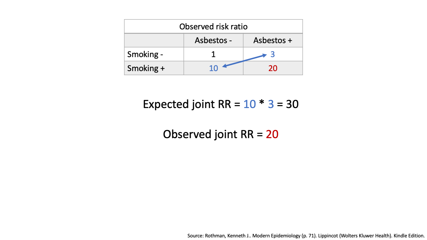
Once again, when there is no effect modification, we expect the combined effects of our two exposures to simply equal the combination of their individual effects. On an multiplicative scale, we combine the individual effects by multiplication.
We already decided that the individual effects of smoking and of asbestos on an multiplicative scale were located in the corners of our table.
We also said that when we are exploring effect modification on an multiplicative scale, we combine the individual effects by multiplication.
Therefore the expected joint risk ratio is 30, which is higher than the observed risk ratio of 20. This is effect modification on the multiplicative scale.
12.4 What is different enough?
Although no clear-cut rule exists regarding whether to adjust in the presence of heterogeneity, consideration of the following question may be helpful: “Given heterogeneity of this magnitude, am I willing to report an average (adjusted) effect that is reasonably representative of all strata of the study population formed on the basis of the suspected effect modifier?”
Again, there is no rule of thumb. It requires subject matter expertise and a certain level of comfort with uncertainty. Would I do anything different based on knowing this? If not, pool.
What should I report?
Additive or multiplicative? Both are important, depending on your question. Therefore, you should often consider reporting information about both additive and multiplicative effect modification.
Both!!! A recent study found only 1 of 50 surveyed epidemiology papers reported information on additive effect modification.
12.5 Key points
- Key concept is effect modification, not effect modifier.
- Effect modification is different than confounding.
- Explore effect modification by:
- Homogeneity of effects
- Observed and expected joint effects
- Can be on an additive or multiplicative scale (or both).
- Can be qualitative or quantitative.
- When there is effect modification, do not pool estimates!