65 Confounding

This chapter is under heavy development and may still undergo significant changes.

Today we are going to talk about confounding bias in epidemiologic studies. I have bias in parentheses here because there is ongoing debate in the field as to whether or not confounding is a type of bias or something that should be considered different than bias. For our purposes, I don’t think it matters much. No matter what we call it, we need to understand it and deal with it.

So, we previously discussed the central role that measurement, typically in the form of data, and data analysis, play in epidemiology. We said that the end result of our measurement and analysis activities typically result in descriptions, predictions, and/or explanations of health-related phenomena.

We also talked about our measures of interest being the result of a combination of the true value and some amount of error in our measurement of that true value.

Then, we talked about breaking down the error in our measurements into two main categories: random error and systematic error.

Then, we talked about breaking down the systematic errors in our measurement into three sources (acknowledging that there may be some overlap). They were: Systematic differences between the population of people we are interested in and the sample of people we are getting measurements from Systematic errors in the way we are taking measurements or collecting data Systematic errors in our estimate of of causal effects due to non-causal (also called spurious) associations.

Last week, we discussed the first two sources of bias. This week, we will discuss the third source of bias – confounding bias, or simply, confounding.

Before discussing more formal definitions of confounding, let’s make sure that we have an intuitive understanding about what confounding is. One classic example used to help people understand confounding is about the relationship between ice cream sales and violent crime.

Remember that one of our definitions for association was, “knowing something about X tells you something about Y, or helps you better predict Y.”

Well, if we go collect a bunch of data on ice cream sales and murder, we will find an association. As ice cream sales increase so do murders, on average.

Data: Ice cream sales (pints per capita) Murders (number) Unadjusted correlation – As ice cream sales increase so do murders, on average.

What are we to make of this? Is there a real relationship between ice cream sales and murder?

Yes. If we know what yesterday’s ice cream sales were, we can really make a better prediction about the number of murders that occurred yesterday, on average.

And the rest of the example goes like this. As the temperature outside rises, people eat more ice cream and murders occur more frequently.

Given this new information, do we still feel as though there a real relationship between ice cream sales and murder?

Yes. If we know what yesterday’s ice cream sales were, we can really make a better prediction about the number of murders that occurred yesterday, on average.

But, is that real relationship causal? No.

Remember one of our definitions of causality. Had X (in this case, ice cream sales) been different and everything else been the same.

Said another way, murders don’t occur more frequently because of ice cream sales. If we increased the price of ice cream to lower sales, would we expect the occurrence of murder to also decline? Most people would say no, of course not.

But, is there anything in our data that can answer that question for us? No. We just all ”know” this somehow. In the world of causal inference, this is known as “expert” knowledge.

As the temperature outside rises: - People eat more ice cream – perhaps to cool off. - Murders are more likely to occur – perhaps because of increases in drug and alcohol use, increases in social mixing, increased irritability due to heat.

Causation: Had X (ice cream sales) been different and everything else been the same. - If we increased the price of ice cream to lower sales, would we expect the occurrence of murder to also decline?

65.1 Ice cream and murder rate simulation

# Load the packages we will need below
library(dplyr, warn.conflicts = FALSE) # The "warn.conflicts" part is optional
library(ggdag, warn.conflicts = FALSE)
library(ggplot2)
library(broom)
library(freqtables)
library(meantables)

We just discussed a classic example of confounding – ice cream sales and murder. Let’s take a look at some simulated data designed to recreate this scenario.

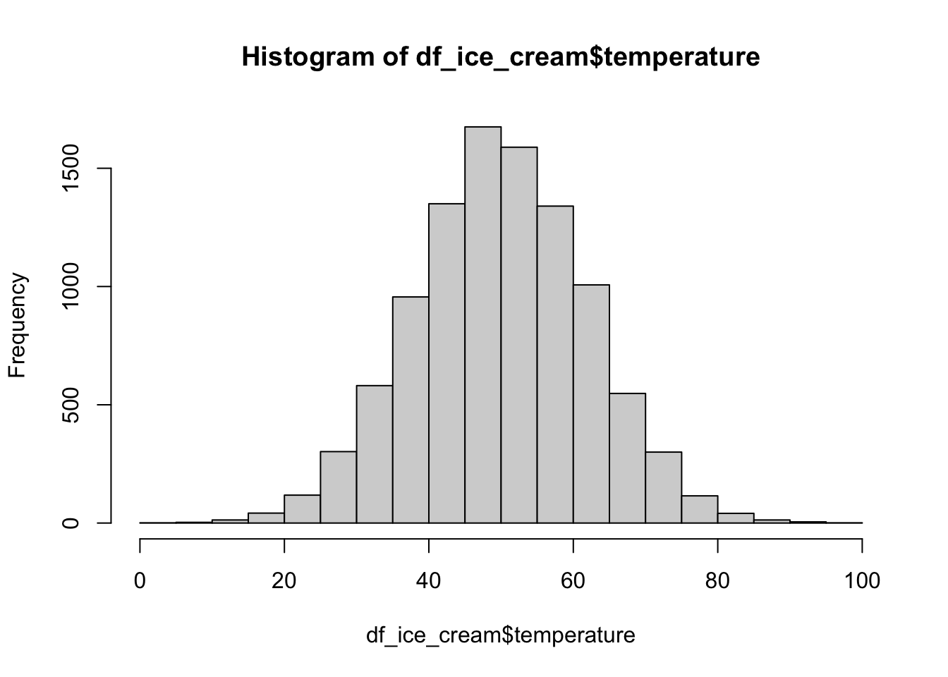
First, we will create temperature. We will make it normally distributed with a mean of 50 and a standard deviation of 12.

# Random number seed so that we can reproduce our results
set.seed(123)

# Sample size
n <- 10000

# Create z - temperature
df_ice_cream <- tibble(temperature = rnorm(n, 50, 12))

And here is what our temperature data looks like in a histogram.

hist(df_ice_cream$temperature)

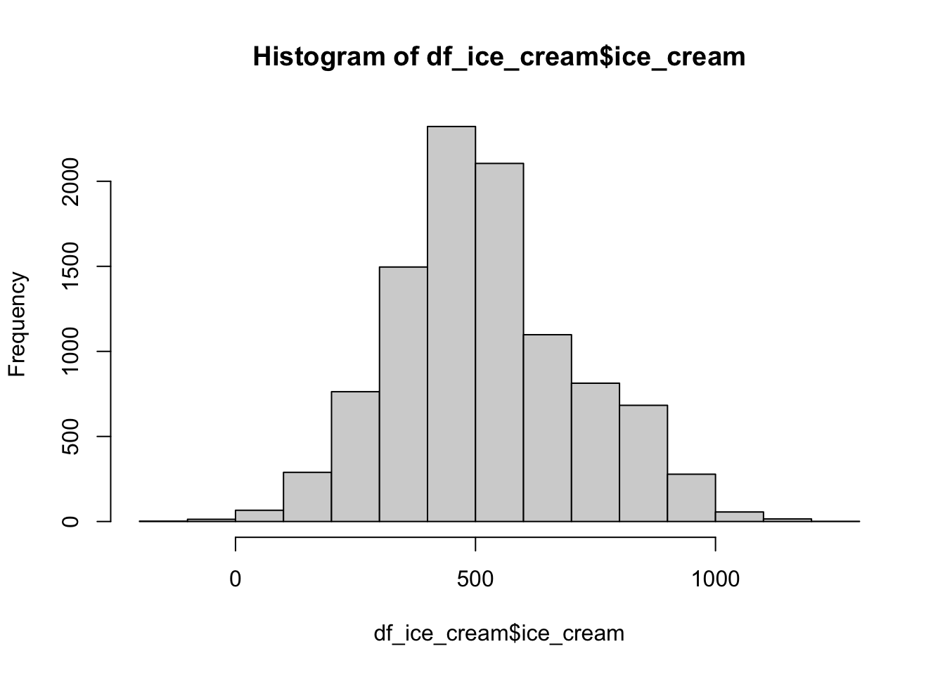
Now, let’s create ice cream sales. In the code below, the values of ice_cream are only determined by our random number generator and the value of temperature. They are totally oblivious to the values of murder. In fact, the murder variable doesn’t even exist yet.

# Set the random number seed so that we can reproduce our results
set.seed(234)

# Set the standard deviation to 100
sd <- 100

# Create a data frame with ice cream sales that are associated with
# temperature
df_ice_cream <- df_ice_cream %>% 
  mutate(
    ice_cream = case_when(
      temperature < 20 ~ rnorm(n, 100, sd),
      temperature < 40 ~ rnorm(n, 300, sd),
      temperature < 60 ~ rnorm(n, 500, sd),
      temperature < 80 ~ rnorm(n, 800, sd),
      temperature < 100 ~ rnorm(n, 1000, sd),
      temperature > 100 ~ rnorm(n, 1200, sd),
    )
  )

And here is what our ice cream sales data looks like in a histogram.

hist(df_ice_cream$ice_cream)

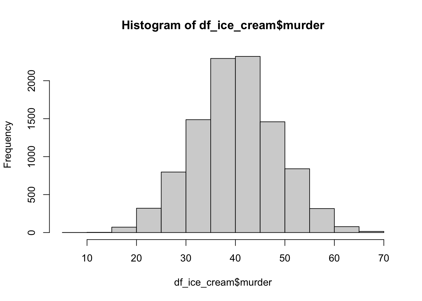
Finally, let’s create the murder variable. In the code below, the values of murder are only determined by our random number generator and the value of temperature. They are totally oblivious to the values of ice cream sales.

# Set the random number seed so that we can reproduce our results
set.seed(456)

# Set the standard deviation to 100
sd <- 5

# Create a data frame with murder rates that are associated with
# temperature
df_ice_cream <- df_ice_cream %>% 
  mutate(
    murder = case_when(
      temperature < 20 ~ rnorm(n, 20, sd),
      temperature < 40 ~ rnorm(n, 30, sd),
      temperature < 60 ~ rnorm(n, 40, sd),
      temperature < 80 ~ rnorm(n, 50, sd),
      temperature < 100 ~ rnorm(n, 60, sd),
      temperature > 100 ~ rnorm(n, 70, sd),
    )
  )

# Change negative murder rates to 0
df_ice_cream <- mutate(df_ice_cream, murder = if_else(murder < 0, 0, murder))

And here is what our murder data looks like in a histogram.

hist(df_ice_cream$murder)

We know that there is no causal relationship between ice_cream and murder because we created them both.

The value of ice_cream is only determined by temperature, not by murders.
The value of murder is only determined by temperature, not by ice cream sales.

Therefore, we might naively expect there to be NO correlation between ice cream sales and murder.

ggplot(df_ice_cream, aes(ice_cream, murder)) + 
  geom_point() + 
  geom_smooth(se = FALSE) + 
  theme_classic()

## `geom_smooth()` using method = 'gam' and formula = 'y ~ s(x, bs = "cs")'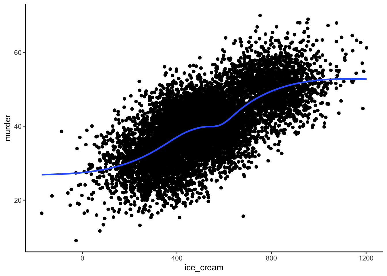

However, there is an obvious correlation between in the data when we view it as a scatter plot. As ice cream sales rise, so do the number of murders, on average.

cor.test(df_ice_cream$ice_cream, df_ice_cream$murder)

## 
##  Pearson's product-moment correlation
## 
## data:  df_ice_cream$ice_cream and df_ice_cream$murder
## t = 90.83, df = 9998, p-value < 0.00000000000000022
## alternative hypothesis: true correlation is not equal to 0
## 95 percent confidence interval:
##  0.6615074 0.6829886
## sample estimates:
##       cor 
## 0.6723896

Further, our Pearson’s correlation coefficient (0.67) indicates that ice cream sales and murder are highly positively correlated in our population.

Again, the association between ice cream sales and murder is a real, valid association. It just doesn’t represent a causal effect. Rather, it’s purely due to the fact that ice cream sales and murder share a common cause – temperature.

And, we can represent that expert knowledge graphically with a DAG.

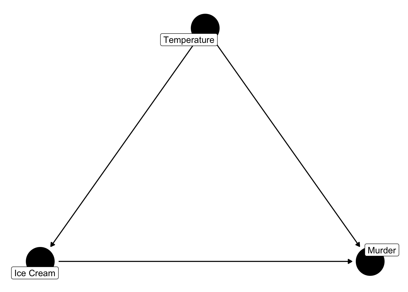
Figure 65.1: Two ice cream and murder DAGs.

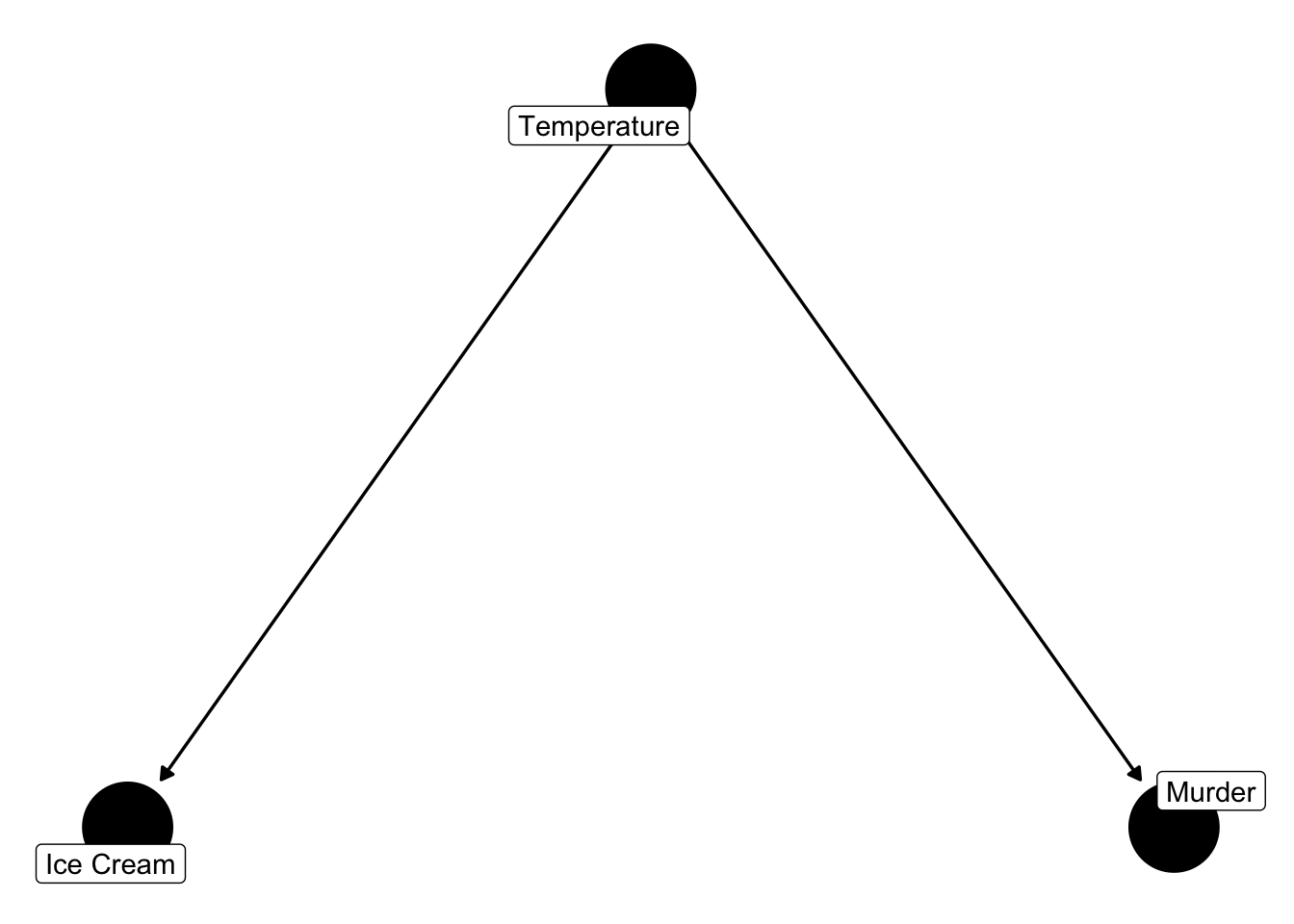
Figure 65.2: Two ice cream and murder DAGs.

In this case, does the DAG on the left or the DAG on the right better represent our assumptions from the previous slide?

The DAG on the right. According to the DAG on the right, ice cream sales do not have a direct causal effect on murder. However, we expect there to be a statistical association between ice cream sales and murder that is due to a common cause of ice cream sales and murder – temperature. Said another way, there is confounding of the null effect of ice cream sales on murder.

At an intuitive level, one of these three explanations of confounding may be helpful to you.

Mixing of effects - Our estimate of the causal effect of ice cream sales on murder was the result of mixing together the effect of temperature and the (null) effect of ice cream sales.

Giving credit to the wrong variable - Saying that our estimate was caused by one variable when, in reality, it was fully or partially caused by another variable. Temperature causes murders to increase, but we gave all the “credit” to ice cream sales.

Influence of another variable - The influence of a third variable distorts an association between exposure and outcome. The true association between ice cream sales and murder is null, but the influence of temperature distorts that association.

Confounding and causal questions

Description: Murders per day. Is that descriptive measure confounded (biased)?

Prediction: Correlation between ice cream sales and murder. Is that predictive measure confounded (biased)?

Explanation: Buying ice cream causes people to murder each other. Is that explanation confounded (biased)?

Earlier I mentioned that there is ongoing discussion in the field about whether or not confounding should be considered a type of bias or something different than bias. I’m not going to attempt to settle that here, but I think it is worth explicitly calling out the fact that confounding is a least special among the biases. Let’s walk through this simple thought experiment.

Assuming no other bias, and a large enough sample size to make random error ignorable:

If we estimate the number of murders per day, do we expect to get a confounded (biased) estimate of murders per day? No.
If we estimate the correlation between ice cream sales and murder and use it to predict future murder rates, do we expect the correlation coefficient to be a confounded (biased) estimate of the association between ice cream sales and murder? No.
If we estimate the correlation between ice cream sales and murder and use it to explain why murder rates increase, do we expect the correlation coefficient to be a confounded (biased) estimate of the causal effect of ice cream sales on murder? Yes.

So, confounding has a special place among the biases, and I think this is because it’s the only bias that requires a causal question to have meaning. What I mean by that is that selection bias or poorly calibrated measurement tools can still create a difference between the truth and your results no matter what the goal of your study is – description, prediction, or causation. For example, estimating murders per day by sampling only affluent suburban neighborhoods would likely lead to a biased descriptive measure of murders anywhere other than affluent suburban neighborhoods.

However, as we saw above, confounding bias requires a causal question to have any real meaning. The mathematical relationship between ice cream sales and violent crime is no more or less interesting than the mathematical relationship, 2 + 2 = 4, in the absence of causal question about the relationship between ice cream sales at violent crime. It’s just a mathematical relationship. As the numbers in column A increase, the numbers in column B tend to also tend to increase. As the numbers in column A decrease, the numbers in column B tend to also decrease, and we can summarize that tendency using a mathematical equation known as a correlation coefficient, for example.

Now that we have an intuitive understanding about what confounding is, what impacts do we expect it to have?

Positive (Away from the null) - Confounder produces observed (unadjusted) estimate of the association between exposure and outcome that is an overestimate of the true (adjusted) association.

For example…

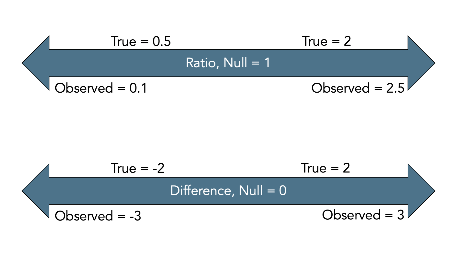
Figure 65.3: Bias away from the null (Positive).

Confounding may also result in estimates that are biased toward the null.

Negative Confounding (Toward the null) - Confounder produces observed (unadjusted) estimate of the association between exposure and outcome that is an underestimate of true (adjusted) association.

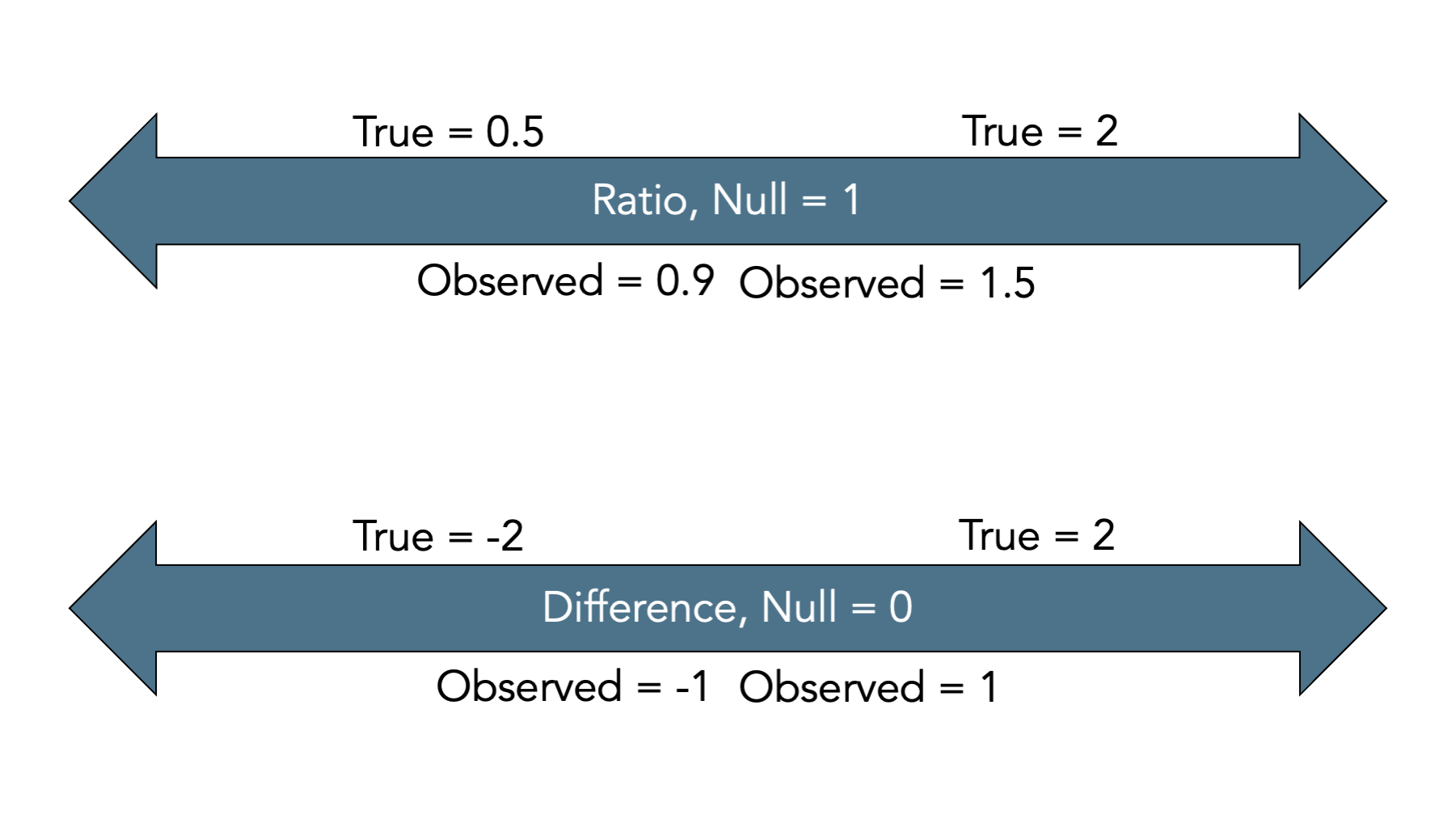
Figure 65.4: Bias toward the null (Negative).

65.2 How do we detect confounding

At this point, we (hopefully) have an intuitive understanding of what confounding is and how it can affect our conclusions. But, how do we know when it exists in our causal effect estimates?

Over the years, methodologist have created different criteria that are intended to tell us if confounding is present. The three we are going to talk about are:

These were also discussed in the Hernan videos, and I think he does a really good job. So, I highly recommend watching those videos if you haven’t already.

Change in estimate criteria
Traditional criteria
Structural criteria

65.2.1 Change in estimate criteria

Calculate an effect measure (OR, RR, etc.) without adjusting for the potential confounder.
Calculate an effect measure (OR, RR, etc.) with adjustment for the potential confounder.
If the the difference between those two measures is greater than or equal to some threshold (usually 10%) then the variable is a confounder.

Borrowing from the Hernan videos…

We expect an association between X and Y even though there is no causal effect of X on Y. If we condition on Z, we expect the association to disappear. This change in the association could easily be 10% or greater. For example OR = 1.2 to OR = 1.0.

In this case, both methods lead us to the same conclusion.

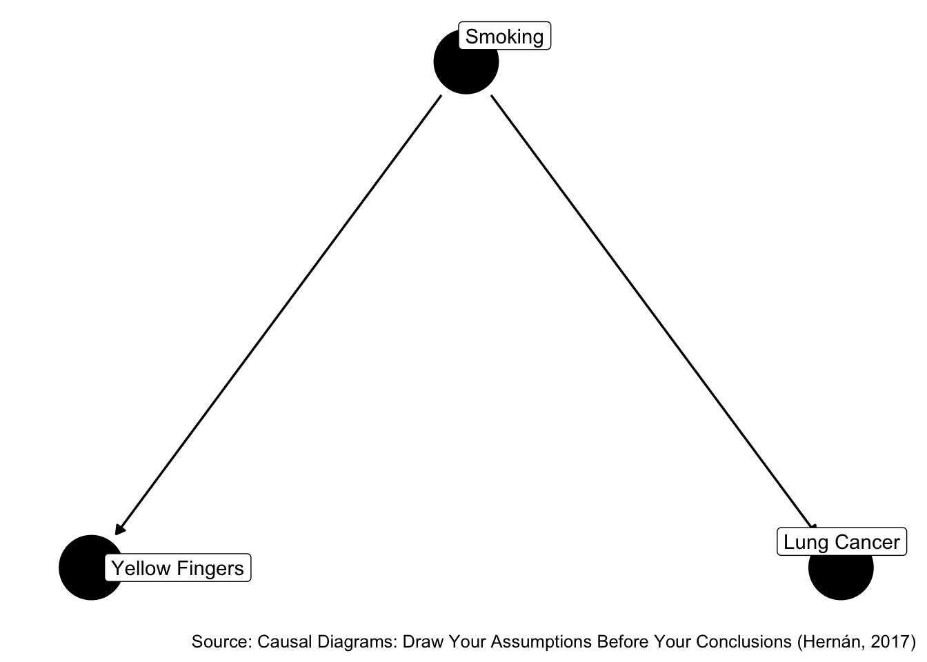
Figure 65.5: Do yellow fingers cause lung cancer?

What about this case, though?

By D-separation, there is no association between X and Z. The null association is an unbiased estimate of the causal effect of Z on X. There is no confounding and therefore, no confounders. However, if we adjust for Y, then the association measure changes. This change in the association could easily be 10% or greater.

The change in estimate criteria would incorrectly lead us to conclude that Y is a confounder. If we use this method, we will label variables as confounders that do not actually help reduce confounding, and possibly even introduce selection bias.

Therefore, we can say that the change in estimate criteria is not sufficient to eliminate confounding.

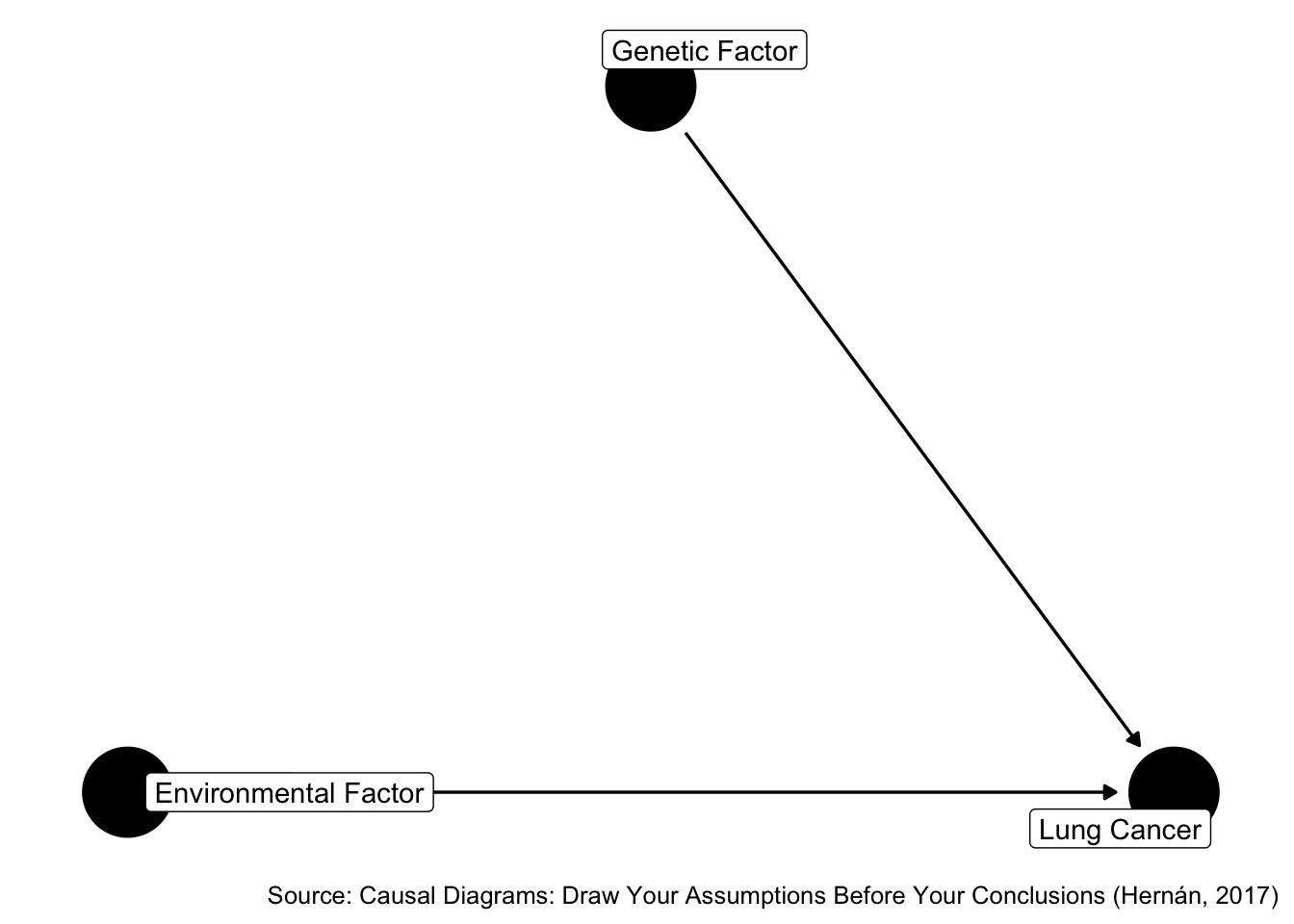
Figure 65.6: Does environmental factor cause and lung cancer?

65.2.2 Traditional criteria

When I was in grad school, I was taught some version of these traditional criteria. There are multiple versions of these criteria. They are all pretty similar. We are going to look at the versions from Szklo and Nieto and the version from Hernan.

Here is the way Szklo and Nieto define those criteria. One issue with Szklo and Nieto version is that it tells us to incorporate information about causal relationships into the criteria for decision making, but gives us no guidance on how to do that.

Therefore, I think comparing Hernan’s version of traditional criteria for confounding with structural criteria for confounding is more useful.

Szklo, M., & Nieto, F. J. (2019), 5.2.1 1. The confounding variable is causally associated with the outcome. 2. The confounding variable is noncausally or causally associated with the exposure. 3. The confounding variable is not in the causal pathway between exposure and outcome.

Hernan (2017) L is a confounder of A and Y if: 1. L is associated with A. 2. L is associated with Y conditional on A (within levels of A). 3. L is not on a causal pathway from A to Y.

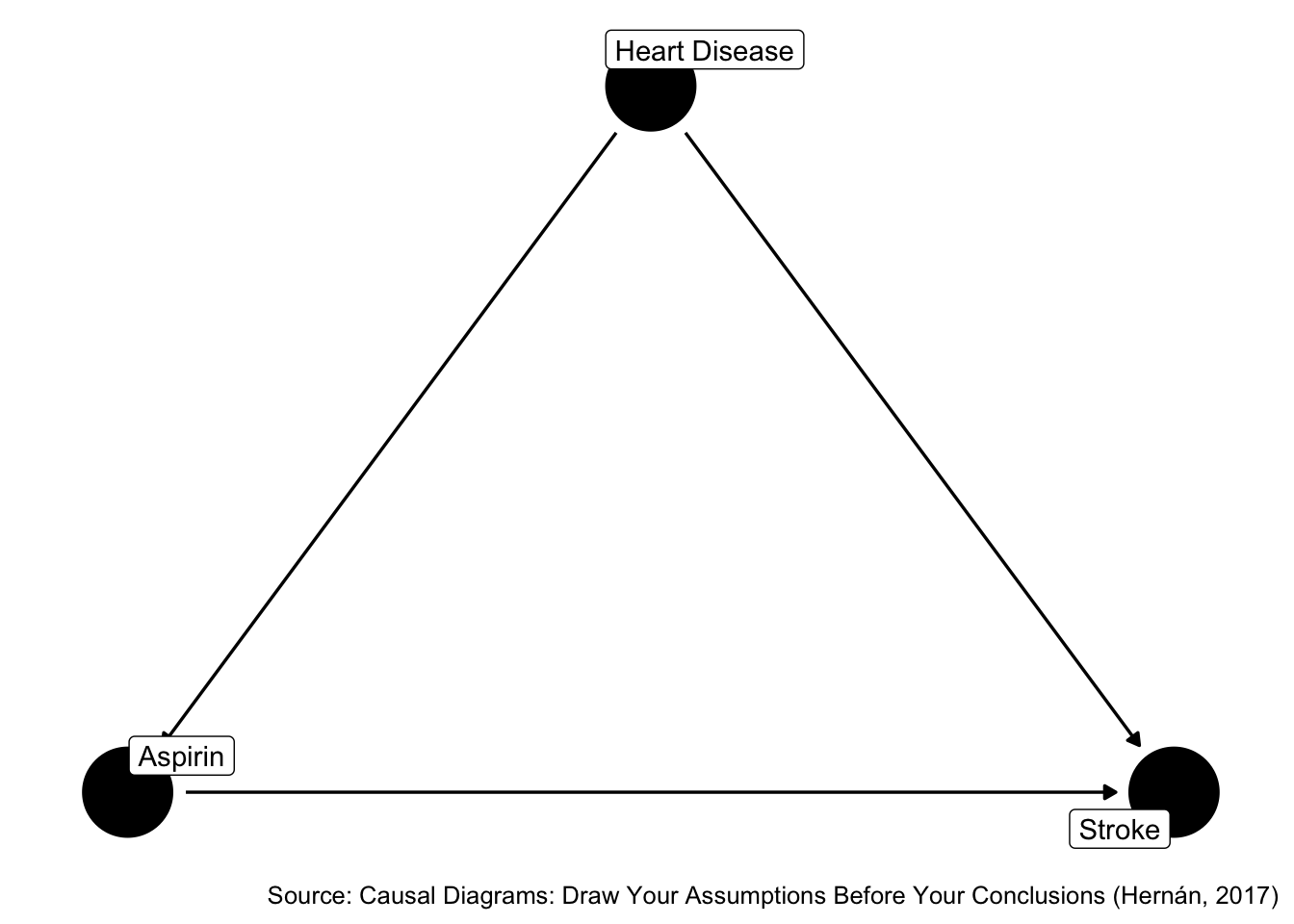
Figure 65.7: Is heart disease a confounder?

Is Z associate with X? Yes. Is Z associated with Y conditional on X? Yes. Is Z in the causal pathway from X to Y? No.

In this case, both methods lead us to the same conclusion. And, as Hernan explains in the videos, we can find lots of examples where the traditional criteria and structural criteria lead us to the same conclusion, but not always…

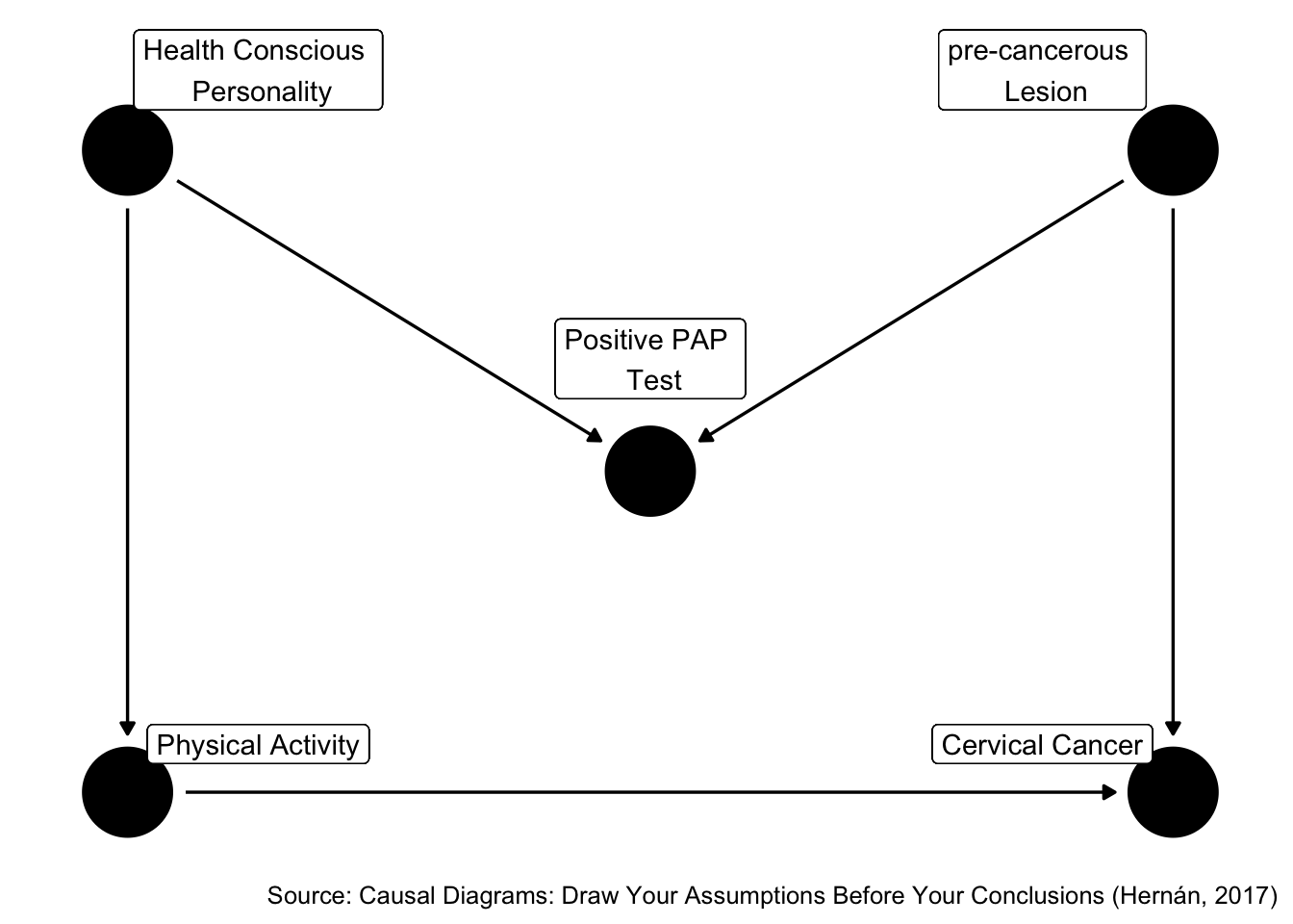
Figure 65.8: Is positive pap test a confounder?

Is Z associate with X? Yes. Is Z associated with Y conditional on X? Yes. Is Z in the causal pathway from X to Y? No.

So, traditional criteria tell us that Z is a confounder, but what do the rules of D-separation tell us?

The traditional criteria would incorrectly lead us to conclude that Z is a confounder. If we use this method, we will label variables as confounders that do not actually help reduce confounding, and possibly even introduce bias.

Therefore, we can say that the traditional criteria is not sufficient to eliminate confounding.

So, what are we left with.

65.2.3 Structural criteria

Current epidemiologic theory tells us that the use of DAGs and structural criteria are the best method currently available to us for identifying and eliminating (where possible) confounding in observational studies.

Let’s walk through this slowly with a little bit of review.

Path: Any arrow-based route between two variables on the graph. Some paths follow the direction of the arrows and some do not.

Some paths follow the direction of the arrows and some do not.

Backdoor path: A backdoor path between X and Y is a path that connects X and Y without using any of the arrows that leave from X.

Figure 65.9: Backdoor paths.

Note: This is NOT the only possible type of backdoor path. See the rules of D-separation.

Backdoor path criterion: We can identify the causal effect of X on Y if we have sufficient data to block all backdoor paths between X and Y.

Emphasis on confounding rather than confounder.

Confounding is a verb, not a noun.

We may call Jill a runner, but that doesn’t imply that she runs 24/7. It just implies that she runs in certain contexts that we deem relevant at the time we call her a runner. In a similar way, SES is not a “confounder.” However, SES may confound causal relationships in certain contexts that we deem relevant when discussing a given topic.

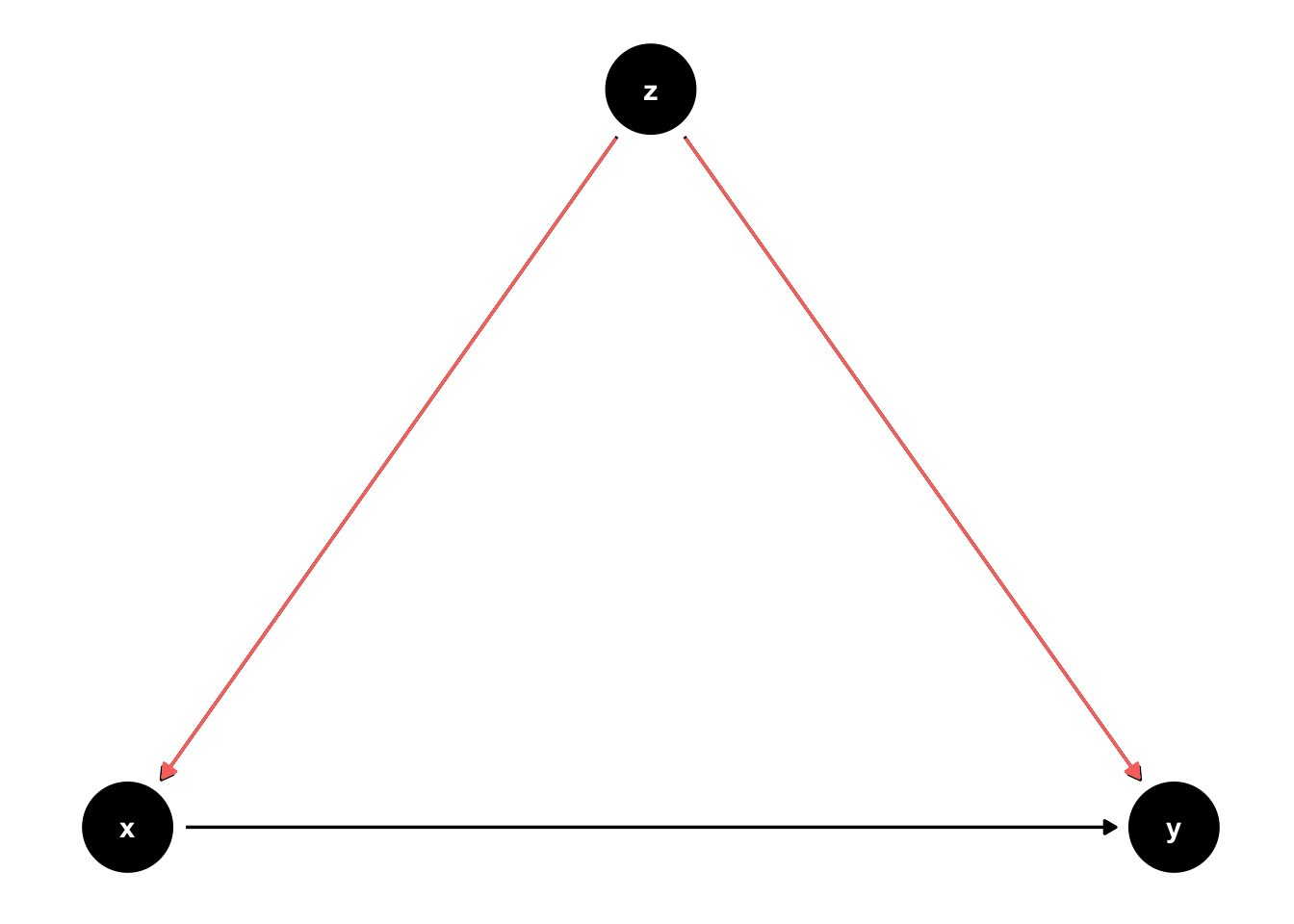
Figure 65.10: Blocking ackdoor paths.

65.3 Confounding

And there are really three equivalent ways we can ask about confounding.

Is there confounding for the effect of X on Y?
Are there any common causes of X on Y?
Are there any open backdoor paths between X and Y?

We can use DAGs, along with the d-separation rules, to answer those questions.