33 Introduction to Repeated Operations
This part of the book is all about the DRY principle. We first discussed the DRY principle in the section on creating and modifying multiple columns. As a reminder, DRY is an acronym for “Don’t Repeat Yourself.” But, what does that mean?
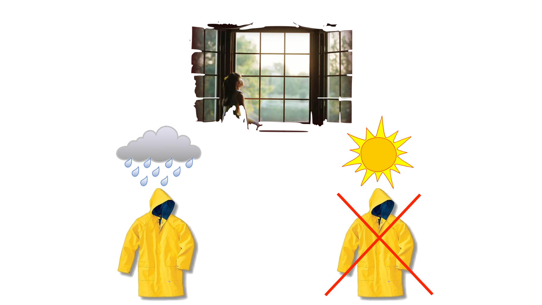
Well, think back to the conditional operations chapter. In that chapter, we compared conditional statements in R with asking our daughters to wear a raincoat if it’s raining. To extend the analogy, now imagine that we wake up one morning and say, “please wear your raincoat if it’s raining today - July 1st.” Then, we wake up the next morning and say, “please wear your raincoat if it’s raining today - July 2nd.” Then, we wake up the next morning and say, “please wear your raincoat if it’s raining today - July 3rd.” And, that pattern continues every morning until our daughters move out of the house. That’s a ton of repetition!! Alternatively, wouldn’t it be much more efficient for me to say, “please wear your raincoat on every day that it rains,” just once?
The same logic applies to our R code. We often want to do the same (or very similar) thing multiple times. This can result in many lines of code that are very similar and unnecessarily repetitive, and this unnecessary repetition can occur in all phases of our projects.
For example:
We may need to write R code to import many different data sets. In such a situation, it isn’t uncommon for the code that imports the data to be the same for each data set – only the file name changes.
We may need to recode certain values in multiple columns of our data frame to missing. In such a situation, it isn’t uncommon for the code that recodes the values to be the same for each column – only the column name changes.
We may need to calculate the same set of statistical measures for many different variables in our data frame. In such a situation, the code to calculate the statistical measures doesn’t change – only the variables being passed to the code.
We may need to create a table of results that includes statistical measures for many different variables in our data frame. In such a situation, the code to prepare and combine the statistical measures into a single table of results doesn’t change – only the variables being passed to the code.
In all of these situations we are asking our R code to do something repeatedly, or iteratively, but with a slight change each time. We can write a separate chunk of code for each time we want to do that thing, or we can write one chunk of code that asks R to do that thing over and over. Writing code in the later way will often result in R programs that:
Are more concise. In other words, we can write one line of code (or relatively few lines of code) instead of many lines of code. Further, such code generally removes “visual clutter” (i.e., the repetitive stuff) that can obscure what the overarching intent of the code.
Contain fewer typos. Every keystroke we make is an opportunity to press the wrong key. If we are writing fewer lines of code, then it logically follows that we are making fewer keystrokes and creating fewer opportunities to hit the wrong key. Similarly, if we are repeatedly copying and pasting code, we are creating opportunities to accidently forget to change a column name, date, file name, etc. in the pasted code.
Are easier to maintain. If we want to change our code, we only have to change it in one place instead of many places. For example, let’s say that we write R code to check the weather every morning. Later, we decide that we want our R code to check the weather and the traffic every morning. Would you rather add that additional request (i.e., check the traffic) to a separate line of code for each day or to the one line of code that asks R to check the weather every day?
🗒Side Note: When I say “one line of code” above, I mean it figuratively. The code we use to remove unnecessary repetition will not necessarily be on one line; however, it should generally require less typing than code that includes unnecessary repetition.
So, writing code that is highly repetitive is usually not a great idea, and this part of the book is all about teaching you to recognize and remove unnecessary repetition from your code. As is often the case with R, there are multiple different methods we can use.
33.1 Multiple methods for repeated operations in R
In the chapters that follow, we will learn four different methods for removing unnecessary repetition from our code. They are:
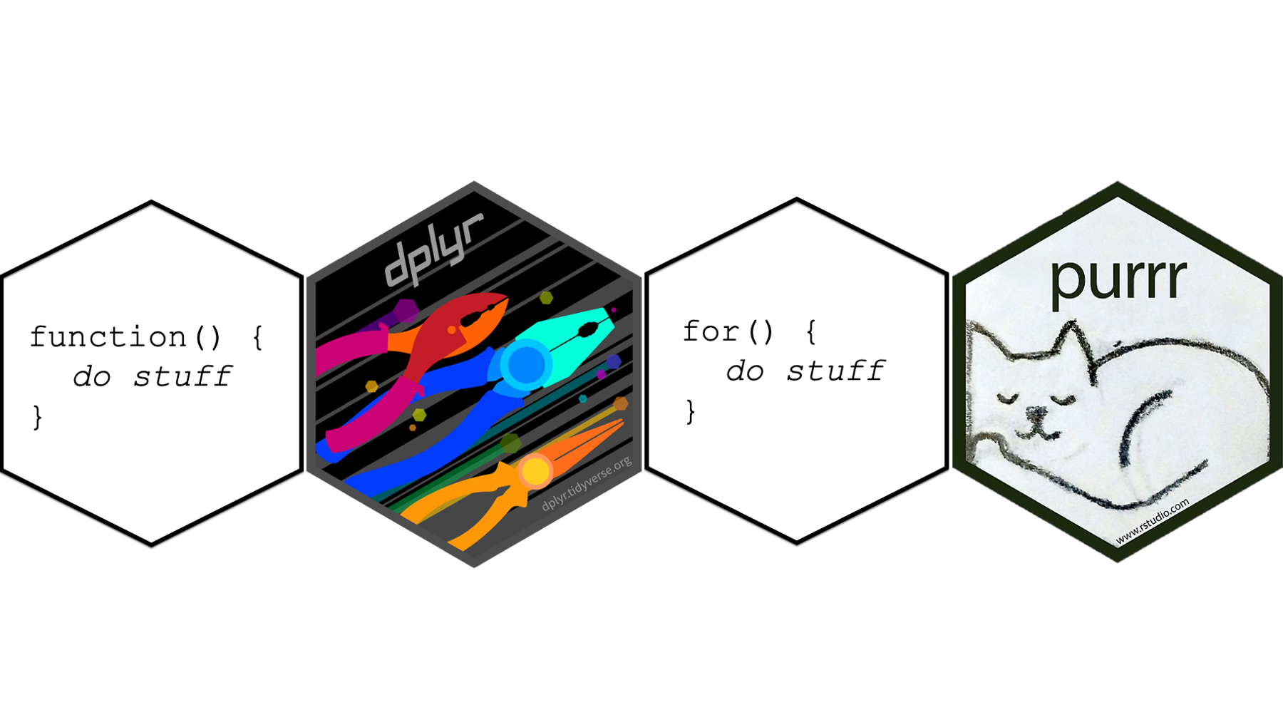
Figure 33.1: Four methods for removing unnecessary repetition.
Writing our own functions that can be reused throughout our code.
Using
dplyr’s column-wise operations.Using for loops.
Using the
purrrpackage.
It’s also important to recognize that each of the methods above can be used independently or in combination with each other. We will see examples of both.
33.2 Tidy evaluation
In case it isn’t obvious to you by now, I’m a fan of the tidyverse packages (i.e., dplyr, ggplot2, tidyr, etc.). I use dplyr, in particular, in virtually every single one of my R programs. The use of non-standard evaluation is just one of the many aspects of the tidyverse packages that I am a fan of. As a reminder, among other things, non-standard evaluation is what allows us to refer to data frame columns without using dollar sign or bracket notation (i.e., data masking). However, non-standard evaluation will create some challenges for us when we try to use functions from tidyverse packages inside of functions and for loops that we write ourselves. Therefore, we will have to learn more about tidy evaluation if we want to continue to use the tidyverse packages that we’ve been using throughout the book so far.
Tidy evaluation can be tricky even for experienced R programmers to wrap their heads around at first. Therefore, I don’t think it will be productive for us to try to learn a lot about the theory behind, or internals of, tidy evaluation as a standalone concept. Instead, in the chapters that follow, I plan to sprinkle in just enough tidy evaluation to accomplish the task at hand. As a little preview, a telltale sign that we are using tidy evaluation will be when you start seeing the {{ (said, curly-curly) operator and the !! (said, bang bang) operator. Hopefully, this will all make more sense in the next chapter when we start to get into some examples.
I recommend the following resources for those of you who are interested in developing a deeper understanding of rlang and tidy evaluation:
Programming with dplyr. Accessed July 31, 2020. https://dplyr.tidyverse.org/articles/programming.html
Wickham H. Introduction. In: Advanced R. Accessed July 31, 2020. https://adv-r.hadley.nz/metaprogramming.html
Now, let’s learn how to write our own functions!🤓