# Performing an operation using a series of steps.
my_numbers <- seq(from = 2, to = 100, by = 2)
my_numbers_logged <- log(my_numbers)
mean_my_numbers_logged <- mean(my_numbers_logged)
mean_my_numbers_logged
[1] 3.662703🤔 What are pipes? This |> is the pipe operator. As of version 4.1, the pipe operator is part of base R. Prior to version 4.1, the pipe operator was only available from the magrittr. The pipe imported from the magrittr package looked like %>% and you may still come across it in R code – including in this book.
🤔 What does the pipe operator do? In our opinion, the pipe operator makes your R code much easier to read and understand.
🤔 How does it do that? It makes your R code easier to read and understand by allowing you to view your nested functions in the order you want them to execute, as opposed to viewing them literally nested inside of each other.
You were first introduced to nesting functions in the Let’s get programming chapter. Recall that functions return values, and the R language allows us to directly pass those returned values into other functions for further calculations. We referred to this as nesting functions and said it was a big deal because it allows us to do very complex operations in a scalable way, without storing a bunch of unneeded intermediate objects in our global environment.
In that chapter, we also discussed a potential downside of nesting functions. Namely, our R code can become really difficult to read when we start nesting lots of functions inside one another.
Pipes allow us to retain the benefits of nesting functions without making our code really difficult to read. At this point, we think it’s best to show you an example. In the code below we want to generate a sequence of numbers, then we want to calculate the log of each of the numbers, and then find the mean of the logged values.
# Performing an operation using a series of steps.
my_numbers <- seq(from = 2, to = 100, by = 2)
my_numbers_logged <- log(my_numbers)
mean_my_numbers_logged <- mean(my_numbers_logged)
mean_my_numbers_logged[1] 3.662703👆 Here’s what we did above:
my_numbers using the seq() function.log() function to create a new vector of numbers called my_numbers_logged, which contains the log values of the numbers in my_numbers.mean() function to create a new vector called mean_my_numbers_logged, which contains the mean of the log values in my_numbers_logged.mean_my_numbers_logged to the screen to view.The obvious first question here is, “why would I ever want to do that?” Good question! You probably won’t ever want to do what we just did in the code chunk above, but we haven’t learned many functions for working with real data yet and we don’t want to distract you with a bunch of new functions right now. Instead, we want to demonstrate what pipes do. So, we’re stuck with this silly example.
👍 What’s nice about the code above? We would argue that it is pretty easy to read because each line does one thing and it follows a series of steps in logical order. First, create the numbers. Second, log the numbers. Third, get the mean of the logged numbers.
👎 What could be better about the code above? All we really wanted was the mean value of the logged numbers (i.e., mean_my_numbers_logged); however, on our way to getting mean_my_numbers_logged we also created two other objects that we don’t care about – my_numbers and my_numbers_logged. It took us time to do the extra typing required to create those objects, and those objects are now cluttering up our global environment. It may not seem like that big of a deal here, but in a real data analysis project these things can really add up.
Next, let’s try nesting these functions instead:
# Performing an operation using nested functions.
mean_my_numbers_logged <- mean(log(seq(from = 2, to = 100, by = 2)))
mean_my_numbers_logged
[1] 3.662703👆Here’s what we did above:
We created a vector of numbers called mean_my_numbers_logged by nesting the seq() function inside of the log() function and nesting the log() function inside of the mean() function.
Then, we printed the value of mean_my_numbers_logged to the screen to view.
👍 What’s nice about the code above? It is certainly more efficient than the sequential step method we used at first. We went from using 4 lines of code to using 2 lines of code, and we didn’t generate any unneeded objects.
👎 What could be better about the code above? Many people would say that this code is harder to read than than the the sequential step method we used at first. This is primarily due to the fact that each line no longer does one thing, and the code no longer follows a sequence of steps from start to finish. For example, the final operation we want to do is calculate the mean, but the mean() function is the first function we see when we read the code.
Finally, let’s try see what this code looks like when we use pipes:
# Performing an operation using pipes.
mean_my_numbers_logged <- seq(from = 2, to = 100, by = 2) |>
  log() |>
  mean()
mean_my_numbers_logged
[1] 3.662703👆Here’s what we did above:
We created a vector of numbers called mean_my_numbers_logged by passing the result of the seq() function directly to the log() function using the pipe operator, and passing the result of the the log() function directly to the mean() function using the pipe operator.
Then, we printed the value of mean_my_numbers_logged to the screen to view.
👏 As you can see, by using pipes we were able to retain the benefits of performing the operation in a series of steps (i.e., each line of code does one thing and they follow in sequential order) and the benefits of nesting functions (i.e., more efficient code).
The utility of the pipe operator may not be immediately apparent to you based on this very simple example. So, next we’re going to show you a little snippet of code from one of our research projects. In the code chunk that follows, the operation we’re trying to perform on the data is written in two different ways – without pipes and with pipes. It’s very unlikely that you will know what this code does, but that isn’t really the point. Just try to get a sense of which version is easier for you to read.
# Nest functions without pipes
responses <- select(ungroup(filter(group_by(filter(merged_data, !is.na(incident_number)), incident_number), row_number() == 1)), date_entered, detect_data, validation)

# Nest functions with pipes
responses <- merged_data |>
  filter(!is.na(incident_number)) |>
  group_by(incident_number) |>
  filter(row_number() == 1) |>
  ungroup() |>
  select(date_entered, detect_data, validation)
What do you think? Even without knowing what this code does, do you feel like one version is easier to read than the other?
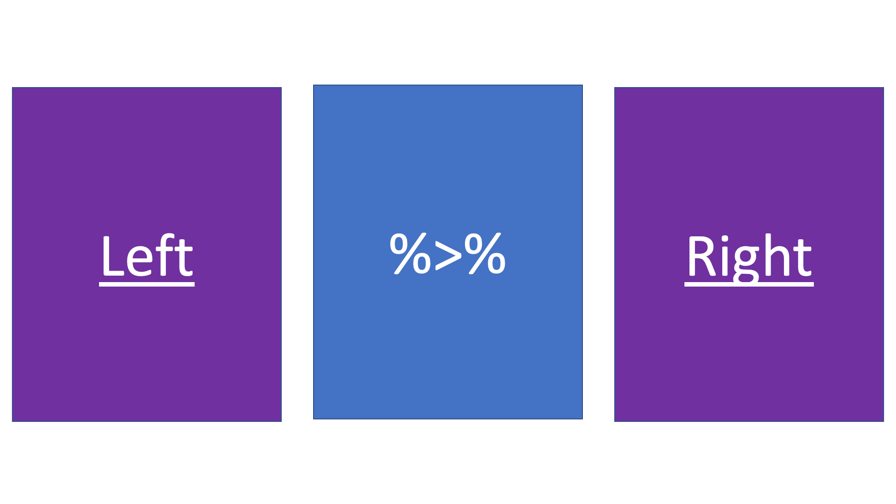
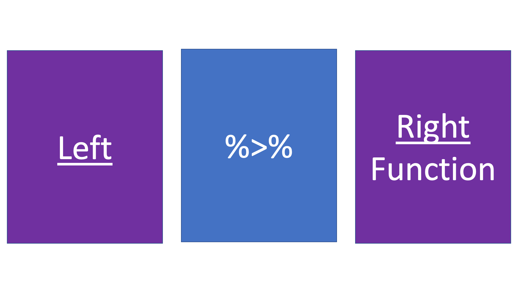
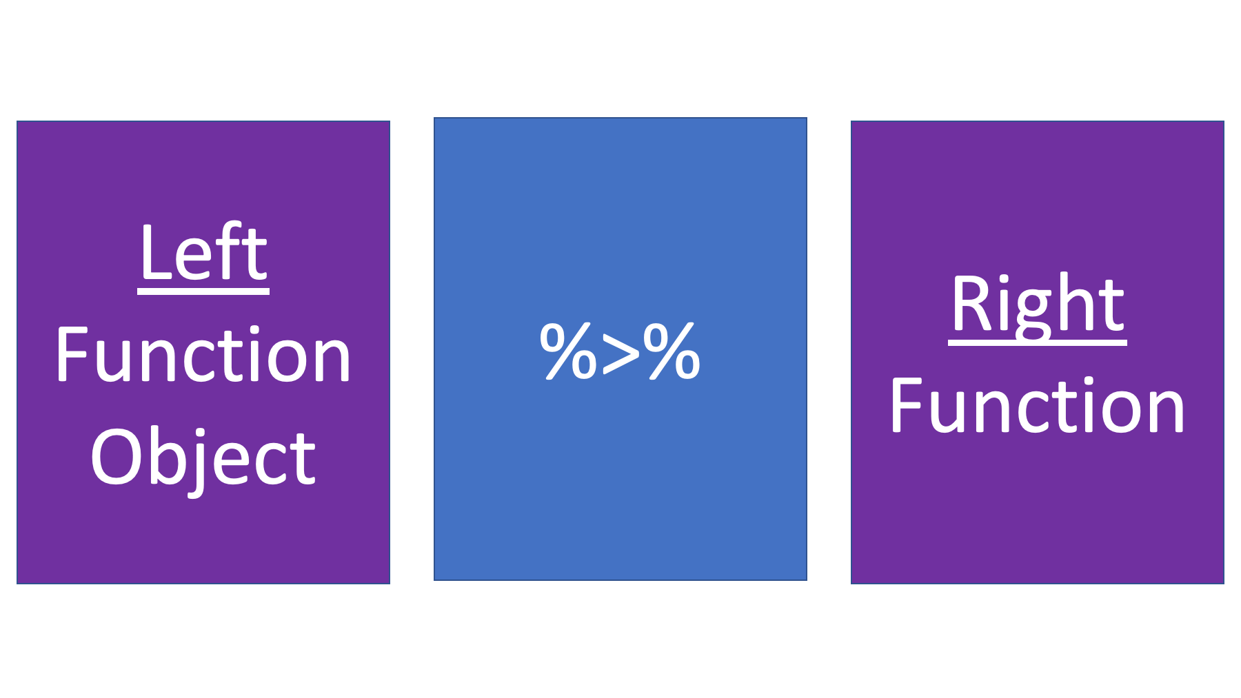
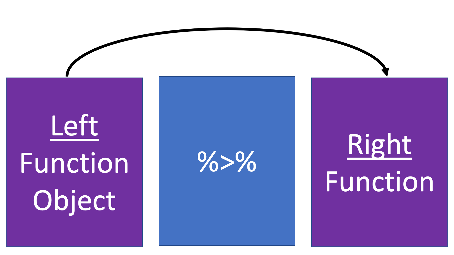
Perhaps we’ve convinced you that pipes are generally useful. But, it may not be totally obvious to you how to use them. They are actually really simple. Start by thinking about pipes as having a left side and a right side.

The thing on the right side of the pipe operator should always be a function.

The thing on the left side of the pipe operator can be a function or an object.

All the pipe operator does is take the thing on the left side and pass it to the first argument of the function on the right side.

It’s a really simple concept, but it can also cause people a lot of confusion at first. So, let’s take look at a couple more concrete examples.
Below we pass a vector of numbers to the to the mean() function, which returns the mean value of those numbers to us.
mean(c(2, 4, 6, 8))[1] 5We can also use a pipe to pass that vector of numbers to the mean() function.
c(2, 4, 6, 8) |> mean()[1] 5So, the R interpreter took the thing on the left side of the pipe operator, stuck it into the first argument of the function on the right side of the pipe operator, and then executed the function. In this case, the mean() function doesn’t require any other arguments, so we don’t have to write anything else inside of the mean() function’s parentheses. When we see c(2, 4, 6, 8) |> mean(), R sees mean(c(2, 4, 6, 8))
Here’s one more example. Pretty soon we will learn how to use the filter() function from the dplyr package to keep only a subset of rows from our data frame. Let’s start by simulating some data:
# Simulate some data
height_and_weight <- tibble(
  id     = c("001", "002", "003", "004", "005"),
  sex    = c("Male", "Male", "Female", "Female", "Male"),
  ht_in  = c(71, 69, 64, 65, 73),
  wt_lbs = c(190, 176, 130, 154, 173)
)

height_and_weight
# A tibble: 5 × 4
id sex ht_in wt_lbs
<chr> <chr> <dbl> <dbl>
1 001 Male 71 190
2 002 Male 69 176
3 003 Female 64 130
4 004 Female 65 154
5 005 Male 73 173In order to work, the filter() function requires us to pass two values to it. The first value is the name of the data frame object with the rows we want to subset. The second is the condition used to subset the rows. Let’s say that we want to do a subgroup analysis using only the females in our data frame. We could use the filter() function like so:
# First value = data frame name (height_and_weight)
# Second value = condition for keeping rows (when the value of sex is Female)
filter(height_and_weight, sex == "Female")
# A tibble: 2 × 4
id sex ht_in wt_lbs
<chr> <chr> <dbl> <dbl>
1 003 Female 64 130
2 004 Female 65 154👆Here’s what we did above:
height_and_weight that had a value of Female for the variable called sex using dplyr’s filter() function.We can also use a pipe to pass the height_and_weight data frame to the filter() function.
# First value = data frame name (height_and_weight)
# Second value = condition for keeping rows (when the value of sex is Female)
height_and_weight |> filter(sex == "Female")
# A tibble: 2 × 4
id sex ht_in wt_lbs
<chr> <chr> <dbl> <dbl>
1 003 Female 64 130
2 004 Female 65 154As you can see, we get the exact same result. So, the R interpreter took the thing on the left side of the pipe operator, stuck it into the first argument of the function on the right side of the pipe operator, and then executed the function. In this case, the filter() function needs a value supplied to two arguments in order to work. So, we wrote sex == "Female" inside of the filter() function’s parentheses. When we see height_and_weight |> filter(sex == "Female"), R sees filter(height_and_weight, sex == "Female").
🗒Side Note: This pattern – a data frame piped into a function, which is usually then piped into one or more additional functions is something that you will see over and over in this book.
Don’t worry too much about how the filter() function works. That isn’t the point here. The two main takeaways so far are:
Pipes make your code easier to read once you get used to them.
The R interpreter knows how to automatically take whatever is on the left side of the pipe operator and make it the value that gets passed to the first argument of the function on the right side of the pipe operator.
Typing |> over and over can be tedious! Thankfully, RStudio provides a keyboard shortcut for inserting the pipe operator into your R code.
On Mac type shift + command + m.
On Windows type shift + control + m
It may not seem totally intuitive at first, but this shortcut is really handy once you get used to it.
As with all the code we write, style is an important consideration. We generally agree with the recommendations given in the Tidyverse style guide. In particular:
We tend to use pipes in such a way that each line of code does one, and only one, thing.
If a line of code contains a pipe operator, the pipe operator should generally be the last thing typed on the line.
The pipe operator should always have a space in front of it.
If the pipe operator isn’t the last thing typed on the line, then it should be have a space after it too.
“If the function you’re piping into has named arguments (like mutate() or summarize()), put each argument on a new line. If the function doesn’t have named arguments (like select() or filter()), keep everything on one line unless it doesn’t fit, in which case you should put each argument on its own line.”1
“After the first step of the pipeline, indent each line by two spaces. RStudio will automatically put the spaces in for you after a line break following a |> . If you’re putting each argument on its own line, indent by an extra two spaces. Make sure ) is on its own line, and un-indented to match the horizontal position of the function name.”1
Each of these recommendations are demonstrated in the code below.
# Do this...
female_height_and_weight <- height_and_weight |> # Line 1
  filter(sex == "Female") |>                     # Line 2
  summarise(                                     # Line 3
    mean_ht = mean(ht_in),                       # Line 4
    sd_ht   = sd(ht_in)                          # Line 5
  ) |>                                           # Line 6
  print()                                        # Line 7
# A tibble: 1 × 2
mean_ht sd_ht
<dbl> <dbl>
1 64.5 0.707In the code above, we would first like you to notice that each line of code does one, and only one, thing. Line 1 only assigns the result of the code pipeline to a new object – female_height_and_weight, line 2 only keeps the rows in the data frame we want – rows for females, line 3 only opens the summarise() function, line 4 only calculates the mean of the ht_in column, line 5 only calculates the standard deviation of the ht_in column, line 6 only closes the summarise() function, and line 7 only prints the result to the screen.
Second, we’d like you to notice that each line containing a pipe operator (i.e., lines 1, 2, and 6) ends with the pipe operator, and the pipe operators all have a space in front of them.
Third, we’d like you to notice that each named argument in the summarise() function is written on its own line (i.e., lines 4 and 5).
Finally, we’d like you notice that each step of the pipeline is indented two spaces (i.e., lines 2, 3, 6, and 7), lines 4 and 5 are indented an additional two spaces because they contain named arguments to the summarise() function, and that the summarise() function’s closing parenthesis is on its own line (i.e., line 6), horizontally aligned with the “s” in “summarise(”.
Now compare that with the code in the code chunk below.
# Avoid this...
female_height_and_weight <- height_and_weight |> filter(sex == "Female") |>
  summarise(mean_ht = mean(ht_in), sd_ht = sd(ht_in)) |> print()
# A tibble: 1 × 2
mean_ht sd_ht
<dbl> <dbl>
1 64.5 0.707Although we get the same result as before, most people would agree that the code is harder to quickly glance at and read. Further, most people would also agree that it would be more difficult to add or rearrange steps when the code is written that way. As previously stated, there is a certain amount of subjectivity in what constitutes “good” style. But, we will once again reiterate that it is important to adopt some style and use it consistently. If you are a beginning R programmer, why not adopt the tried-and-true styles suggested here and adjust later if you have a compelling reason to do so?
We think it’s important to note that not everyone in the R programming community is a fan of using pipes. We hope that we’ve made a compelling case for why we use pipes, but we acknowledge that it is ultimately a preference, and that using pipes is not the best choice in all circumstances. Whether or not you choose to use the pipe operator is up to you; however, we will be using them extensively throughout the remainder of this book.